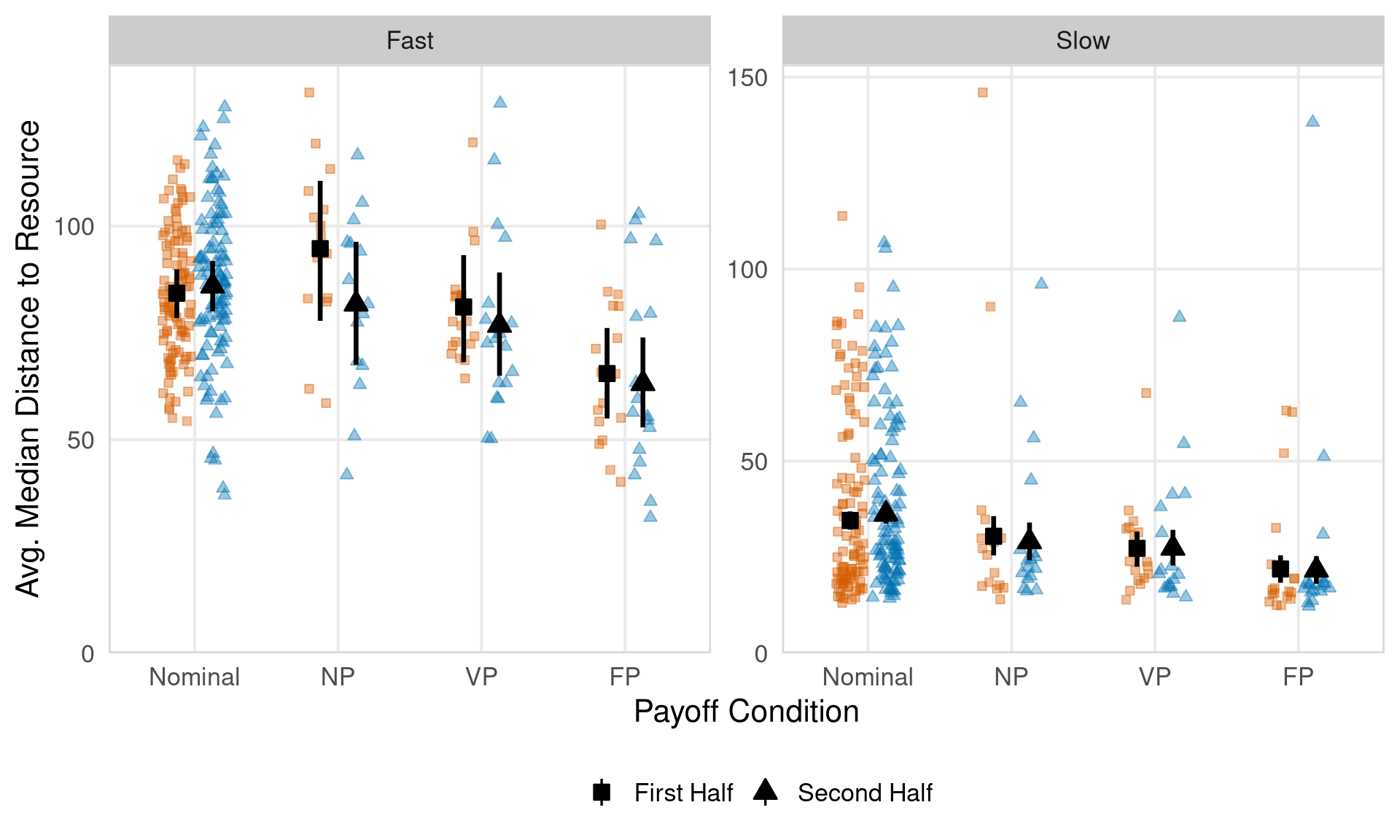
Average Median Distance to Resource by Epoch
We now duplicate the analysis above but calculating the average median distance
separately for the first half (time <= 440) and second half (time > 440) of the
study, adding Epoch as an interaction term to the model.
Statistical Model (Epoch)
Model specification
m.AvgMedDist.2.formula <- brmsformula(
  AvgMedDist ~ 1 + SignalingType * ResourceSpeed * Epoch + (1 | Group),
  family = Gamma(link = "log")
)

m.AvgMedDist.2.formula_comparison <- brmsformula(
  AvgMedDist ~ 1 + SignalingType * ResourceSpeed * Epoch
)

m.AvgMedDist.2.priors <-
  prior(normal(0, 0.5), class = b) +
  prior(normal(4, 1), class = Intercept) +
  prior(gamma(4, 0.1), class = shape) +
  prior(exponential(1), class = sd, lb = 0)
Model fitting
m.AvgMedDist.2.fit <- brm(
  formula = m.AvgMedDist.2.formula,
  data = m.AvgMedDist.epoch.model_data,
  prior = m.AvgMedDist.2.priors,
  chains = 7,
  cores = 7,
  seed = 42,
  iter = 10000,
  file = paste0(fits_path, "avg_med_dist_2.rds"),
  backend = "cmdstanr",
  threads = threading(100),
  control = list(adapt_delta = 0.99),
  save_pars = save_pars(all = TRUE)
)
## Family: gamma
## Links: mu = log; shape = identity
## Formula: AvgMedDist ~ 1 + SignalingType * ResourceSpeed * Epoch + (1 | Group)
## Data: m.AvgMedDist.epoch.model_data (Number of observations: 622)
## Draws: 7 chains, each with iter = 10000; warmup = 5000; thin = 1;
## total post-warmup draws = 35000
##
## Multilevel Hyperparameters:
## ~Group (Number of levels: 311)
## Estimate Est.Error l-95% CI u-95% CI Rhat Bulk_ESS Tail_ESS
## sd(Intercept) 0.33 0.02 0.30 0.37 1.00 10401 19251
##
## Regression Coefficients:
## Estimate Est.Error l-95% CI u-95% CI Rhat Bulk_ESS Tail_ESS
## Intercept 4.43 0.04 4.35 4.51 1.00 10128 17903
## SignalingTypeNP 0.11 0.11 -0.11 0.33 1.00 10876 17814
## SignalingTypeVP -0.04 0.10 -0.24 0.16 1.00 11265 17647
## SignalingTypeFP -0.26 0.11 -0.46 -0.05 1.00 10668 18733
## ResourceSpeedslow -0.89 0.06 -1.01 -0.78 1.00 9235 17183
## EpochSecondHalf 0.02 0.04 -0.05 0.09 1.00 19077 24705
## SignalingTypeNP:ResourceSpeedslow -0.24 0.15 -0.54 0.06 1.00 10521 16714
## SignalingTypeVP:ResourceSpeedslow -0.20 0.15 -0.48 0.09 1.00 10833 18321
## SignalingTypeFP:ResourceSpeedslow -0.20 0.15 -0.49 0.08 1.00 10693 17785
## SignalingTypeNP:EpochSecondHalf -0.17 0.10 -0.36 0.03 1.00 21402 25665
## SignalingTypeVP:EpochSecondHalf -0.07 0.09 -0.25 0.10 1.00 21707 25977
## SignalingTypeFP:EpochSecondHalf -0.06 0.10 -0.24 0.13 1.00 20779 22983
## ResourceSpeedslow:EpochSecondHalf 0.03 0.05 -0.07 0.13 1.00 18136 24883
## SignalingTypeNP:ResourceSpeedslow:EpochSecondHalf 0.07 0.14 -0.20 0.34 1.00 20607 25735
## SignalingTypeVP:ResourceSpeedslow:EpochSecondHalf 0.03 0.13 -0.23 0.29 1.00 21460 24828
## SignalingTypeFP:ResourceSpeedslow:EpochSecondHalf -0.00 0.13 -0.26 0.26 1.00 20514 23506
##
## Further Distributional Parameters:
## Estimate Est.Error l-95% CI u-95% CI Rhat Bulk_ESS Tail_ESS
## shape 13.83 1.08 11.81 16.02 1.00 15029 23742
##
## Draws were sampled using sample(hmc). For each parameter, Bulk_ESS
## and Tail_ESS are effective sample size measures, and Rhat is the potential
## scale reduction factor on split chains (at convergence, Rhat = 1).Condition comparisons
m.AvgMedDist.2.emmeans_contrast_draws.1 <- m.AvgMedDist.2.fit %>%
  emmeans(~ SignalingType * ResourceSpeed * Epoch,
    epred = TRUE,
    type = "response",
    re_formula = m.AvgMedDist.2.formula_comparison
  ) %>%
  contrast(method = "revpairwise", by = c("SignalingType", "ResourceSpeed"), combine = TRUE) %>%
gather_emmeans_draws()m.AvgMedDist.2.comparison.1 <- m.AvgMedDist.2.emmeans_contrast_draws.1 %>%
ggdist::mean_hdci(.width = 0.9) %>%
mutate(.value = round(.value, 2), .lower = round(.lower, 2), .upper = round(.upper, 2))
m.AvgMedDist.2.comparison.1 %>%
filter(!is.na(contrast)) %>%
knitr::kable("html", digits = 2) %>%
kable_classic(full_width = TRUE, position = "center")| contrast | SignalingType | ResourceSpeed | .value | .lower | .upper | .width | .point | .interval |
|---|---|---|---|---|---|---|---|---|
| Second Half - First Half | Nominal | fast | 1.70 | -3.47 | 6.79 | 0.9 | mean | hdci |
| Second Half - First Half | Nominal | slow | 1.67 | -0.59 | 3.84 | 0.9 | mean | hdci |
| Second Half - First Half | NP | fast | -12.95 | -26.89 | 1.04 | 0.9 | mean | hdci |
| Second Half - First Half | NP | slow | -1.39 | -5.83 | 3.27 | 0.9 | mean | hdci |
| Second Half - First Half | VP | fast | -4.27 | -15.26 | 6.76 | 0.9 | mean | hdci |
| Second Half - First Half | VP | slow | 0.06 | -4.12 | 4.39 | 0.9 | mean | hdci |
| Second Half - First Half | FP | fast | -2.34 | -11.84 | 7.18 | 0.9 | mean | hdci |
| Second Half - First Half | FP | slow | -0.26 | -3.51 | 3.01 | 0.9 | mean | hdci |
Condition comparison table (Epoch)
m.AvgMedDist.2.comparison.table <- m.AvgMedDist.2.comparison.1 %>%
  filter(!is.na(contrast)) %>%
  select(ResourceSpeed, SignalingType, contrast, .value, .lower, .upper) %>%
  mutate(
    ResourceSpeed = ifelse(is.na(ResourceSpeed), ".", as.character(ResourceSpeed)),
    SignalingType = ifelse(is.na(SignalingType), ".", as.character(SignalingType)),
    sig = (.lower * .upper) > 0,
    Estimate = sprintf("%.2f", .value),
    Estimate = ifelse(sig, paste0("\\textbf{", Estimate, "}"), Estimate),
    hpdi = sprintf("[%.2f, %.2f]", .lower, .upper),
    hpdi = ifelse(sig, paste0("\\textbf{", hpdi, "}"), hpdi)
  ) %>%
  select(ResourceSpeed, SignalingType, contrast, Estimate, hpdi) %>%
  mutate(contrast = "Second - First Half")

colnames(m.AvgMedDist.2.comparison.table) <- c(
  "Resource Speed", "Payoff Condition", "Contrast", "Mean", "90\\% HPDI"
)

kbl_epoch <- kable(
  m.AvgMedDist.2.comparison.table,
  format = "latex",
  booktabs = TRUE,
  align = c("l", "l", "l", "r", "r"),
  caption = "Posterior Estimates Average Median Distance by Epoch",
  escape = FALSE
) %>%
  kable_styling(latex_options = "hold_position") %>%
  row_spec(0, bold = TRUE)

unique_speeds_epoch <- unique(m.AvgMedDist.2.comparison.table$`Resource Speed`)
start <- 1
for (speed in unique_speeds_epoch) {
  n_rows <- sum(m.AvgMedDist.2.comparison.table$`Resource Speed` == speed)
  if (speed != ".") {
    kbl_epoch <- group_rows(kbl_epoch, speed, start, start + n_rows - 1)
  }
  start <- start + n_rows
}

writeLines(kbl_epoch, paste0(comparisons, "avg_med_dist_2_comparison.tex"))