Tracking Efficiency
theoretical_max <- 40
m.PCR.data <- subj_data %>%
  select(Participant, Group, ResourceSpeed, SignalingType, PCS) %>%
  mutate(PCS_0_1 = PCS / theoretical_max)
PCS distribution by conditions
m.PCR.data %>%
  ggplot(aes(x = PCS)) +
  geom_histogram(binwidth = 2, fill = "lightblue", color = "black") +
  facet_grid(rows = vars(ResourceSpeed), cols = vars(SignalingType)) +
  theme_nice()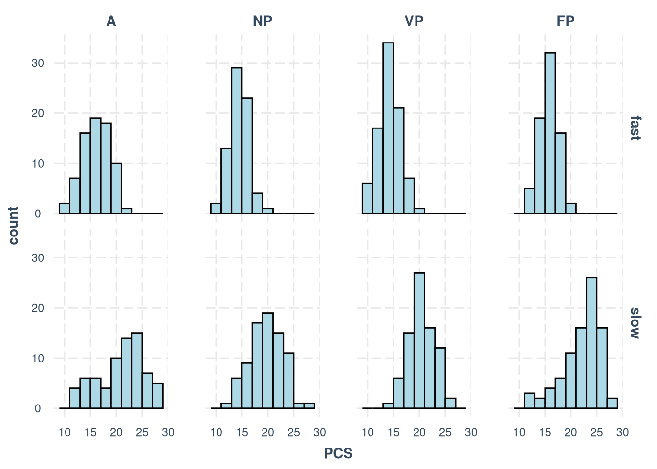
# Check if PCS can be exactly 0 or 40
m.PCR.data %>%
  filter(PCS == 0 | PCS == theoretical_max) %>%
  select(Participant, PCS, ResourceSpeed, SignalingType)
Model 1
m.PCR.1.formula <- brmsformula(
  PCS_0_1 ~ 1 + SignalingType * ResourceSpeed + (1 | Group),
  family = Beta(link = "logit", link_phi = "log")
  )

m.PCR.1.formula_comparison <- brmsformula(
  PCS_0_1 ~ 1 + SignalingType * ResourceSpeed
  )

m.PCR.1.priors <-
    prior(normal(0, 0.5), class = b) +
    prior(normal(0, 1), class = Intercept) +
    prior(normal(2, 1), class = phi, lb = 0) +
prior(normal(0, 1), class = sd, lb = 0)Prior predictive checks
m.PCR.1.fit_prior <- brm(
  formula = m.PCR.1.formula,
  data    = m.PCR.data,
  prior   = m.PCR.1.priors,
  chains  = 4,
  cores   = 4,
  seed    = 42,
  iter    = 2000,
  file = paste0(fits_path, 'pcr_1_prior.rds'),
  sample_prior = "only",
  backend = "cmdstanr",
  threads = threading(100),
  control = list(adapt_delta = 0.95),
  save_pars = save_pars(all = TRUE))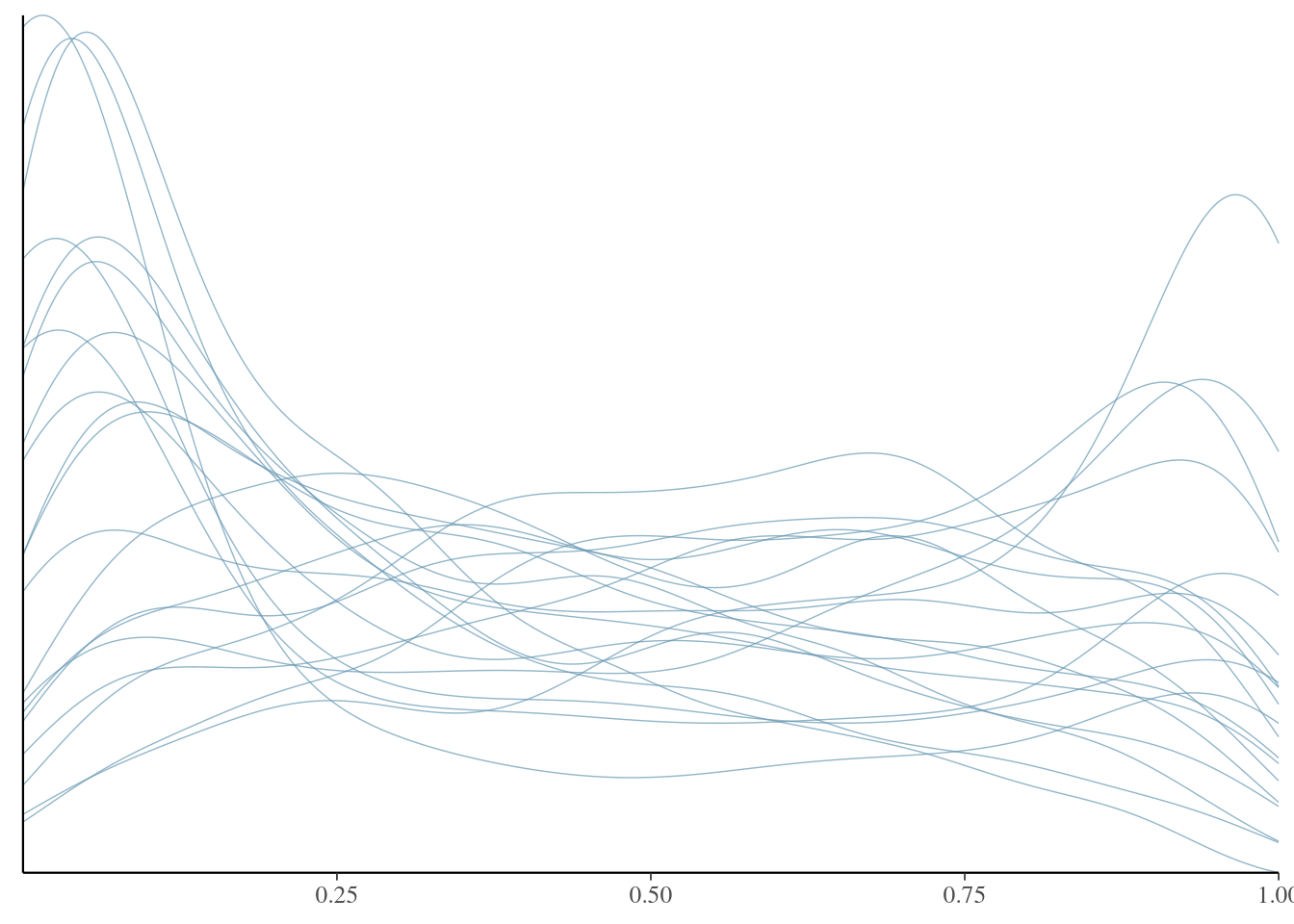
##  Family: beta
##   Links: mu = logit; phi = identity
## Formula: PCS_0_1 ~ 1 + SignalingType * ResourceSpeed + (1 | Group)
##    Data: m.PCR.data (Number of observations: 621)
##   Draws: 4 chains, each with iter = 2000; warmup = 1000; thin = 1;
##          total post-warmup draws = 4000
##
## Multilevel Hyperparameters:
## ~Group (Number of levels: 247)
##               Estimate Est.Error l-95% CI u-95% CI Rhat Bulk_ESS Tail_ESS
## sd(Intercept)     0.81      0.61     0.03     2.27 1.00     2689     1541
##
## Regression Coefficients:
##                                   Estimate Est.Error l-95% CI u-95% CI Rhat Bulk_ESS Tail_ESS
## Intercept                            -0.03      1.07    -2.10     2.00 1.00     9375     3250
## SignalingTypeNP                      -0.00      0.50    -0.98     0.95 1.00     6094     2949
## SignalingTypeVP                      -0.00      0.51    -0.97     0.98 1.00     7254     2724
## SignalingTypeFP                       0.00      0.48    -0.95     0.94 1.00     7907     2798
## ResourceSpeedslow                    -0.00      0.49    -0.95     0.95 1.00     6907     2629
## SignalingTypeNP:ResourceSpeedslow     0.01      0.49    -0.92     0.95 1.00     7112     3016
## SignalingTypeVP:ResourceSpeedslow    -0.01      0.50    -1.00     0.95 1.00     7115     2901
## SignalingTypeFP:ResourceSpeedslow     0.00      0.50    -0.97     0.97 1.00     7420     2709
##
## Further Distributional Parameters:
##     Estimate Est.Error l-95% CI u-95% CI Rhat Bulk_ESS Tail_ESS
## phi     2.06      0.94     0.34     3.94 1.00     2856     1397
##
## Draws were sampled using sample(hmc). For each parameter, Bulk_ESS
## and Tail_ESS are effective sample size measures, and Rhat is the potential
## scale reduction factor on split chains (at convergence, Rhat = 1).
Model fitting
m.PCR.1.fit <- brm(
  formula = m.PCR.1.formula,
  data    = m.PCR.data,
  prior   = m.PCR.1.priors,
  chains  = 7,
  cores   = 7,
  seed    = 42,
  iter    = 20000,
  file = paste0(fits_path, 'pcr_1.rds'),
  backend = "cmdstanr",
  threads = threading(100),
  control = list(adapt_delta = 0.95),
  save_pars = save_pars(all = TRUE)
)## Family: beta
## Links: mu = logit; phi = identity
## Formula: PCS_0_1 ~ 1 + SignalingType * ResourceSpeed + (1 | Group)
## Data: m.PCR.data (Number of observations: 621)
## Draws: 7 chains, each with iter = 20000; warmup = 10000; thin = 1;
## total post-warmup draws = 70000
##
## Multilevel Hyperparameters:
## ~Group (Number of levels: 247)
## Estimate Est.Error l-95% CI u-95% CI Rhat Bulk_ESS Tail_ESS
## sd(Intercept) 0.03 0.02 0.00 0.07 1.00 44768 36289
##
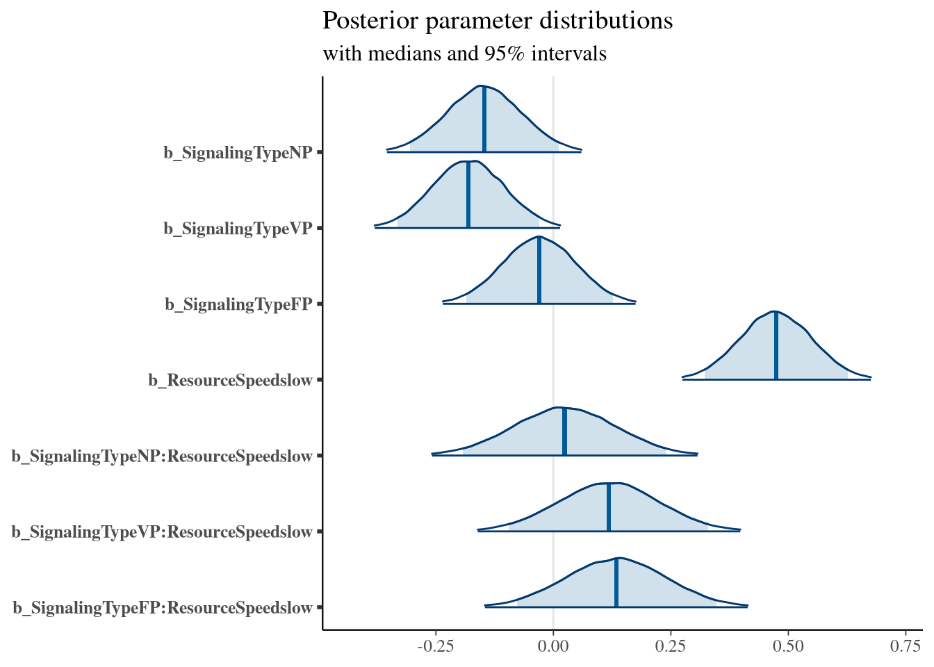
## Regression Coefficients:
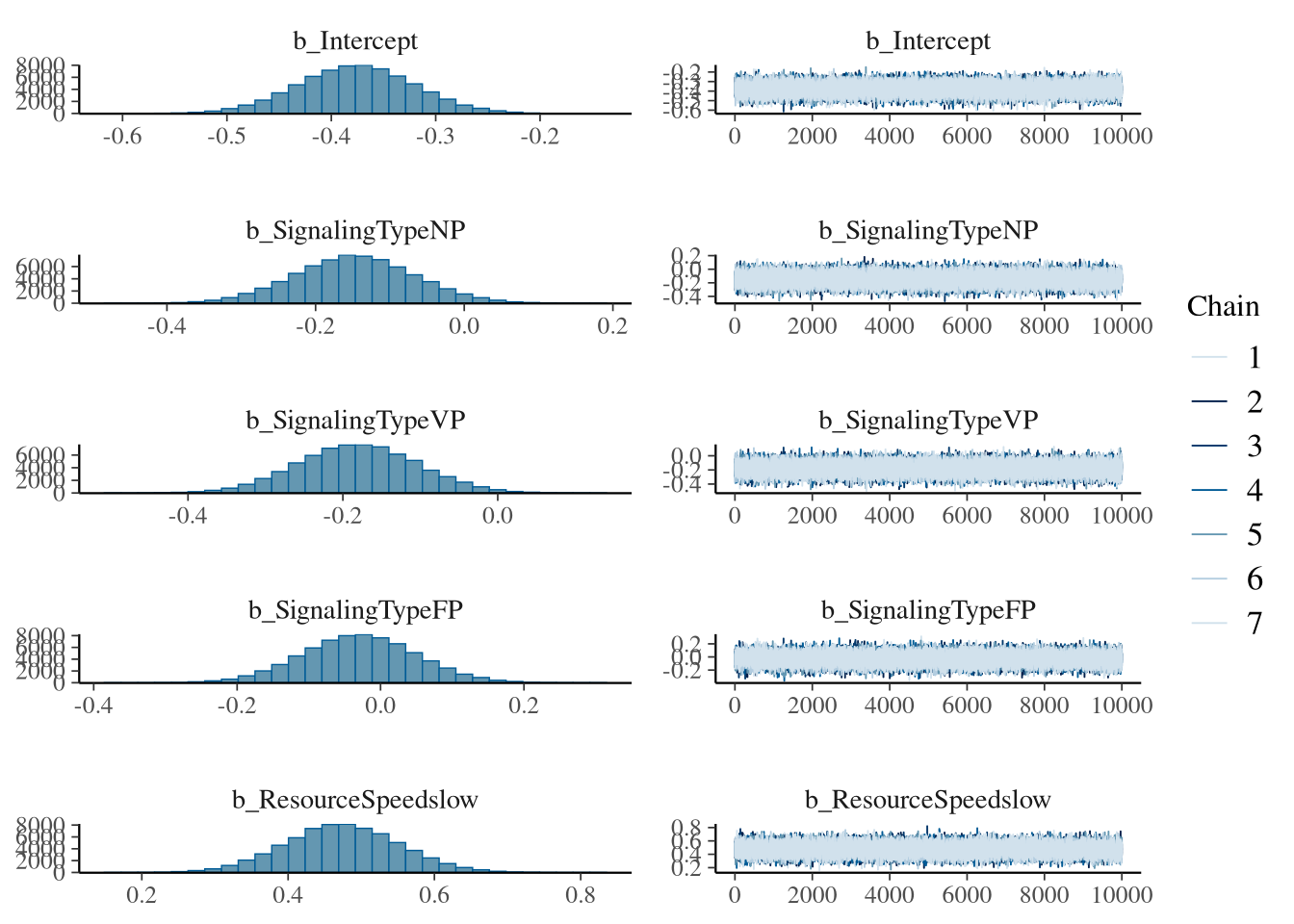
## Estimate Est.Error l-95% CI u-95% CI Rhat Bulk_ESS Tail_ESS
## Intercept -0.38 0.06 -0.49 -0.27 1.00 55301 56556
## SignalingTypeNP -0.15 0.08 -0.31 0.01 1.00 68325 57564
## SignalingTypeVP -0.18 0.08 -0.33 -0.03 1.00 67324 59737
## SignalingTypeFP -0.03 0.08 -0.19 0.13 1.00 64695 56519
## ResourceSpeedslow 0.47 0.08 0.32 0.63 1.00 49826 54319
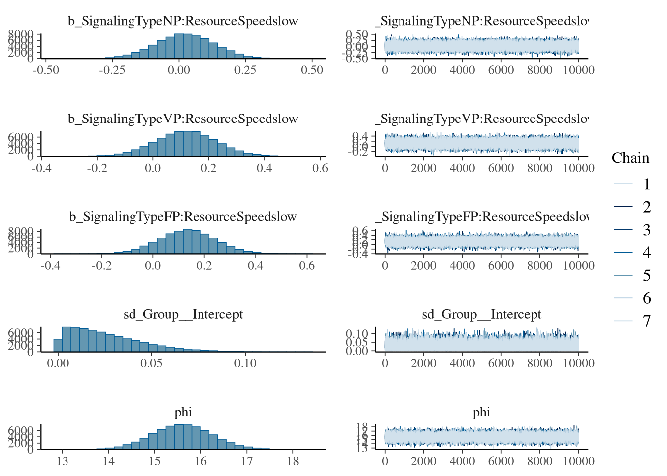
## SignalingTypeNP:ResourceSpeedslow 0.02 0.11 -0.19 0.24 1.00 60986 57926
## SignalingTypeVP:ResourceSpeedslow 0.12 0.11 -0.10 0.33 1.00 60422 57596
## SignalingTypeFP:ResourceSpeedslow 0.13 0.11 -0.08 0.35 1.00 58708 56643
##
## Further Distributional Parameters:
## Estimate Est.Error l-95% CI u-95% CI Rhat Bulk_ESS Tail_ESS
## phi 15.61 0.66 14.33 16.91 1.00 177705 47876
##
## Draws were sampled using sample(hmc). For each parameter, Bulk_ESS
## and Tail_ESS are effective sample size measures, and Rhat is the potential
## scale reduction factor on split chains (at convergence, Rhat = 1).Model diagnostics
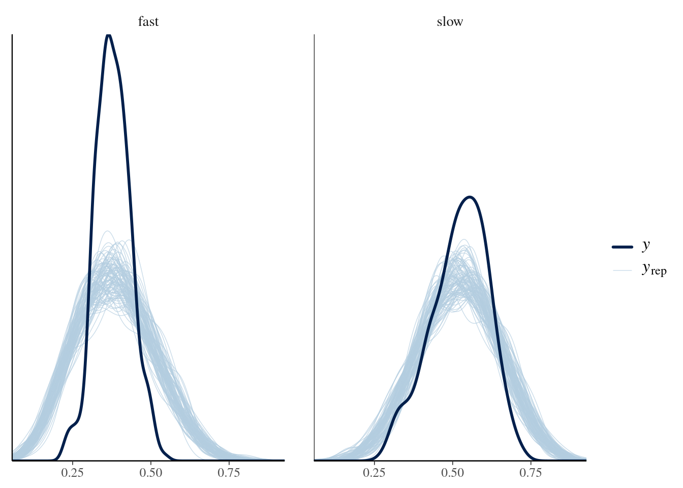
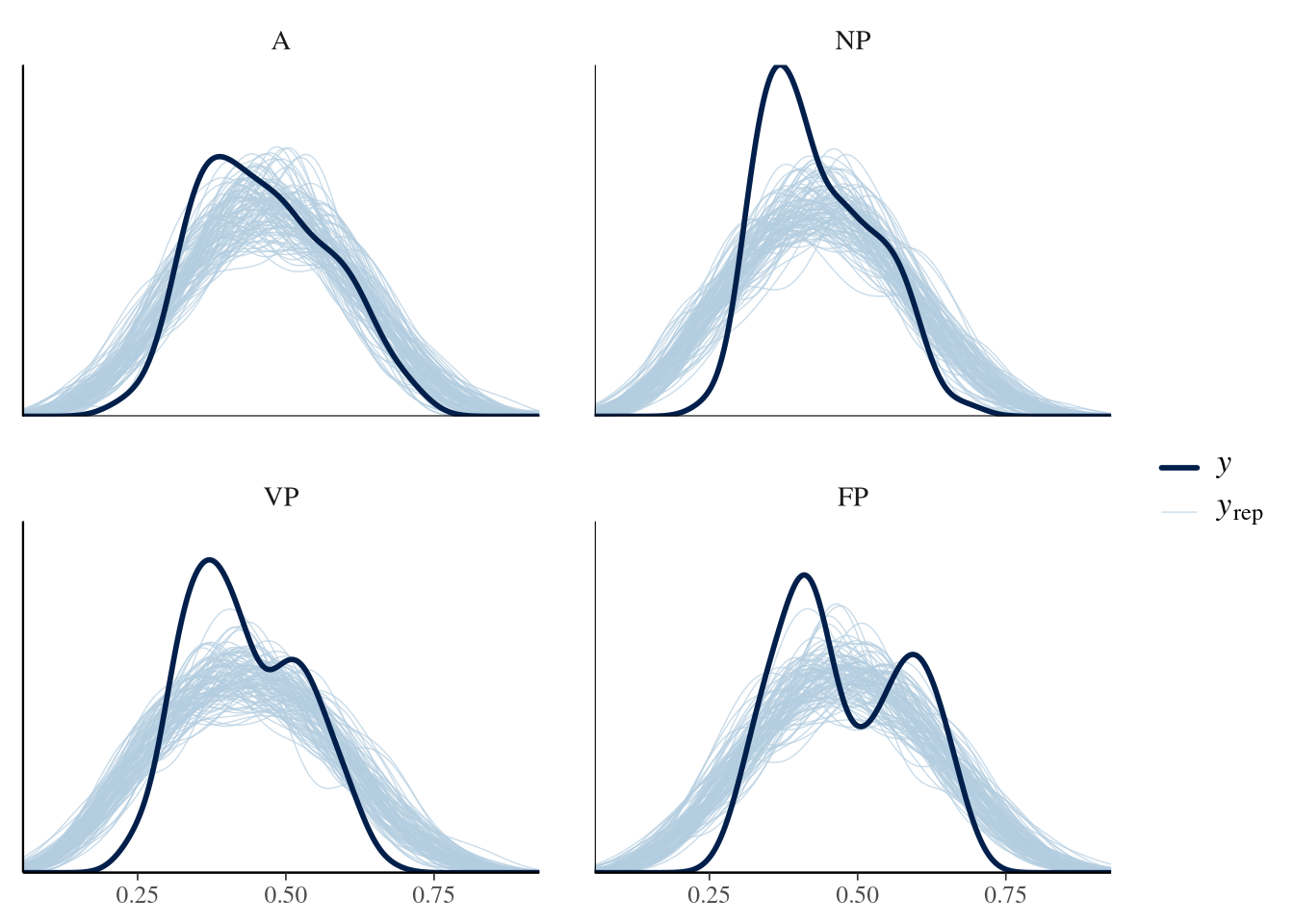
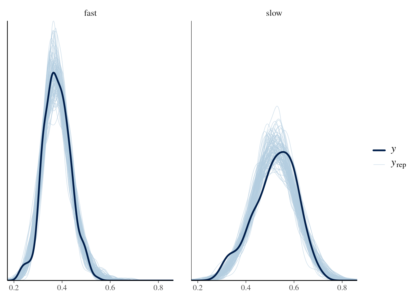
group <- m.PCR.data$SignalingType
mask <- m.PCR.data$ResourceSpeed == 'fast'

ppc_dens_overlay_grouped(m.PCR.1.y[mask],
                         m.PCR.1.yrep[1:50, mask],
                         group = group[mask])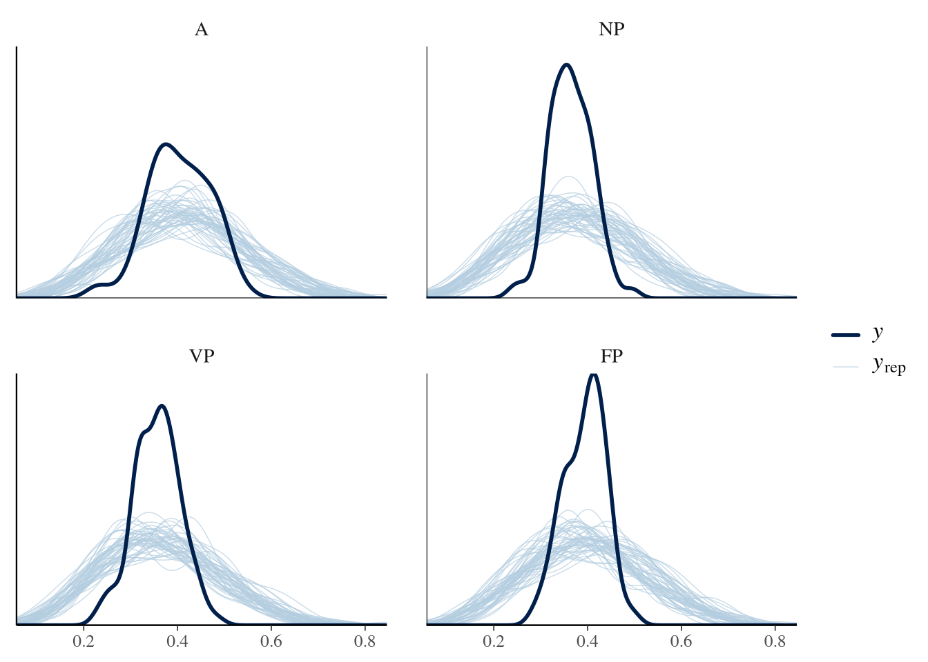
group <- m.PCR.data$SignalingType
mask <- m.PCR.data$ResourceSpeed == 'slow'

ppc_dens_overlay_grouped(m.PCR.1.y[mask],
                         m.PCR.1.yrep[1:50, mask],
                         group = group[mask])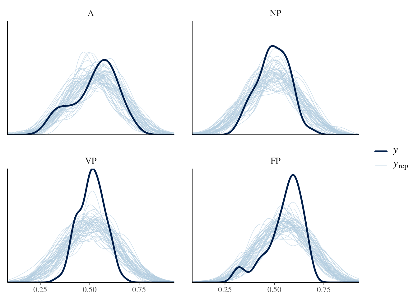
Condition comparisons
m.PCR.1.emmeans_contrast_draws.1 <- m.PCR.1.fit %>%
  emmeans(~ SignalingType * ResourceSpeed, epred = TRUE, type = "response", re_formula = m.PCR.1.formula_comparison) %>%
  contrast(method = "revpairwise", simple = "each", combine = TRUE) %>%
  gather_emmeans_draws() %>%
mutate(.value = .value * theoretical_max)m.PCR.1.comparison.1 <- m.PCR.1.emmeans_contrast_draws.1 %>%
ggdist::mean_hdci(.width = 0.9) %>%
mutate(.value = round(.value, 2), .lower = round(.lower, 2), .upper = round(.upper, 2))
m.PCR.1.comparison.1 %>%
knitr::kable("html", digits = 2) %>% kable_classic(full_width = T, position = "center", )| ResourceSpeed | SignalingType | contrast | .value | .lower | .upper | .width | .point | .interval |
|---|---|---|---|---|---|---|---|---|
| . | A | slow - fast | 4.69 | 3.43 | 5.95 | 0.9 | mean | hdci |
| . | FP | slow - fast | 6.01 | 4.76 | 7.26 | 0.9 | mean | hdci |
| . | NP | slow - fast | 4.86 | 3.60 | 6.16 | 0.9 | mean | hdci |
| . | VP | slow - fast | 5.77 | 4.54 | 7.00 | 0.9 | mean | hdci |
| fast | . | FP - A | -0.29 | -1.54 | 0.96 | 0.9 | mean | hdci |
| fast | . | FP - NP | 1.11 | -0.19 | 2.40 | 0.9 | mean | hdci |
| fast | . | FP - VP | 1.42 | 0.20 | 2.67 | 0.9 | mean | hdci |
| fast | . | NP - A | -1.40 | -2.67 | -0.14 | 0.9 | mean | hdci |
| fast | . | VP - A | -1.71 | -2.90 | -0.50 | 0.9 | mean | hdci |
| fast | . | VP - NP | -0.31 | -1.58 | 0.92 | 0.9 | mean | hdci |
| slow | . | FP - A | 1.03 | -0.24 | 2.31 | 0.9 | mean | hdci |
| slow | . | FP - NP | 2.26 | 1.01 | 3.51 | 0.9 | mean | hdci |
| slow | . | FP - VP | 1.66 | 0.40 | 2.91 | 0.9 | mean | hdci |
| slow | . | NP - A | -1.23 | -2.53 | 0.06 | 0.9 | mean | hdci |
| slow | . | VP - A | -0.63 | -1.94 | 0.66 | 0.9 | mean | hdci |
| slow | . | VP - NP | 0.61 | -0.68 | 1.88 | 0.9 | mean | hdci |
m.PCR.1.emmeans_contrast_draws.1 %>%
  filter(ResourceSpeed != '.') %>%
  rename(prediction = .value) %>%
  ggplot(
    aes(y = contrast,
        x = prediction,
        color = ResourceSpeed, shape = ResourceSpeed, fill = ResourceSpeed)) +
  facet_grid(rows = vars(ResourceSpeed)) +
  stat_pointinterval(.width = 0.9) +
  scale_color_manual(values = get_colors("Qual2", num.colors = 2, reverse = TRUE, gradient = FALSE)) +
  scale_fill_manual(values = get_colors("Qual2", num.colors = 2, reverse = TRUE, gradient = FALSE)) +
  scale_shape_manual(values = c(21, 24)) +
  labs(x = 'Prediction PCS') +
  theme_nice()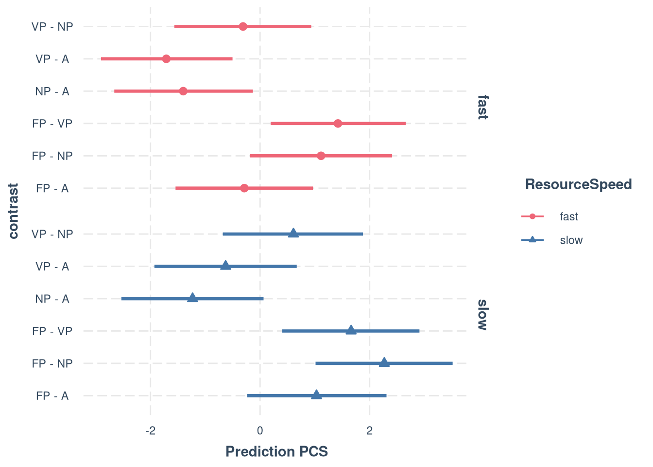
m.PCR.1.emmeans_contrast_draws.2 <- m.PCR.1.fit %>%
  emmeans(~ ResourceSpeed, epred = TRUE, type = "response", re_formula = m.PCR.1.formula_comparison) %>%
  contrast(method = "revpairwise", simple = "each", combine = TRUE) %>%
  gather_emmeans_draws() %>%
mutate(.value = .value * theoretical_max)m.PCR.1.comparison.2 <- m.PCR.1.emmeans_contrast_draws.2 %>%
ggdist::mean_hdci(.width = 0.9) %>%
mutate(.value = round(.value, 2), .lower = round(.lower, 2), .upper = round(.upper, 2))
m.PCR.1.comparison.2 %>%
knitr::kable("html", digits = 2) %>% kable_classic(full_width = T, position = "center", )| contrast | .value | .lower | .upper | .width | .point | .interval |
|---|---|---|---|---|---|---|
| slow - fast | 5.33 | 4.69 | 5.98 | 0.9 | mean | hdci |
Model 2
m.PCR.2.formula <- brmsformula(
  PCS_0_1 ~ 1 + SignalingType * ResourceSpeed + (1 | Group),
  phi ~ ResourceSpeed + SignalingType,
  family = Beta(link = "logit", link_phi = "log")
  )

m.PCR.2.formula_comparison <- brmsformula(
  PCS_0_1 ~ 1 + SignalingType * ResourceSpeed,
  phi ~ ResourceSpeed + SignalingType
  )

m.PCR.2.priors <-
    prior(normal(0, 0.5), class = b) +
    prior(normal(0, 1), class = Intercept) +
    prior(gamma(4, 0.1), class = Intercept, dpar = phi, lb = 0) +
    prior(normal(0, 1), class = b, dpar = phi) +
prior(normal(0, 1), class = sd, lb = 0)Prior predictive checks
m.PCR.2.fit_prior <- brm(
  formula = m.PCR.2.formula,
  data    = m.PCR.data,
  prior   = m.PCR.2.priors,
  chains  = 4,
  cores   = 4,
  seed    = 42,
  iter    = 2000,
  file = paste0(fits_path, 'pcr_2_prior.rds'),
  sample_prior = "only",
  backend = "cmdstanr",
  threads = threading(100),
  control = list(adapt_delta = 0.95),
  save_pars = save_pars(all = TRUE))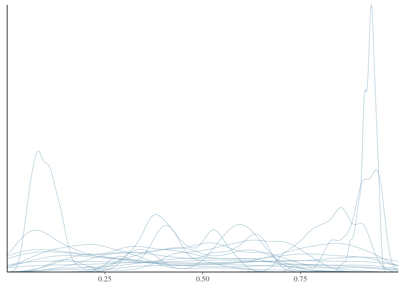
##  Family: beta
##   Links: mu = logit; phi = log
## Formula: PCS_0_1 ~ 1 + SignalingType * ResourceSpeed + (1 | Group)
##          phi ~ ResourceSpeed + SignalingType
##    Data: m.PCR.data (Number of observations: 621)
##   Draws: 4 chains, each with iter = 2000; warmup = 1000; thin = 1;
##          total post-warmup draws = 4000
##
## Multilevel Hyperparameters:
## ~Group (Number of levels: 247)
##               Estimate Est.Error l-95% CI u-95% CI Rhat Bulk_ESS Tail_ESS
## sd(Intercept)     0.79      0.60     0.03     2.24 1.00     3113     1560
##
## Regression Coefficients:
##                                   Estimate Est.Error l-95% CI u-95% CI Rhat Bulk_ESS Tail_ESS
## Intercept                             0.01      1.03    -2.08     2.01 1.00     5691     3085
## phi_Intercept                        39.42     20.96    10.02    88.07 1.00     4885     2501
## SignalingTypeNP                       0.00      0.48    -0.94     0.95 1.00     4813     3051
## SignalingTypeVP                      -0.00      0.51    -0.99     1.02 1.00     5656     3220
## SignalingTypeFP                       0.01      0.50    -0.96     1.01 1.00     4794     2830
## ResourceSpeedslow                     0.00      0.49    -0.96     0.96 1.00     4946     2946
## SignalingTypeNP:ResourceSpeedslow    -0.01      0.51    -1.01     0.98 1.00     5189     2931
## SignalingTypeVP:ResourceSpeedslow    -0.00      0.50    -0.96     1.00 1.00     5035     2984
## SignalingTypeFP:ResourceSpeedslow    -0.00      0.51    -1.00     0.99 1.00     5284     2328
## phi_ResourceSpeedslow                 0.01      0.98    -1.94     1.98 1.00     4825     3045
## phi_SignalingTypeNP                  -0.01      1.01    -2.02     1.99 1.00     4741     2870
## phi_SignalingTypeVP                   0.01      0.99    -1.90     1.89 1.00     5314     2739
## phi_SignalingTypeFP                   0.01      1.01    -1.99     2.03 1.00     5061     3248
##
## Draws were sampled using sample(hmc). For each parameter, Bulk_ESS
## and Tail_ESS are effective sample size measures, and Rhat is the potential
## scale reduction factor on split chains (at convergence, Rhat = 1).
Model fitting
m.PCR.2.fit <- brm(
  formula = m.PCR.2.formula,
  data    = m.PCR.data,
  prior   = m.PCR.2.priors,
  chains  = 7,
  cores   = 7,
  seed    = 42,
  iter    = 20000,
  file = paste0(fits_path, 'pcr_2.rds'),
  backend = "cmdstanr",
  threads = threading(100),
  control = list(adapt_delta = 0.95),
  save_pars = save_pars(all = TRUE)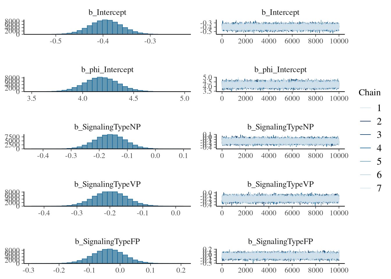
)## Family: beta
## Links: mu = logit; phi = log
## Formula: PCS_0_1 ~ 1 + SignalingType * ResourceSpeed + (1 | Group)
## phi ~ ResourceSpeed + SignalingType
## Data: m.PCR.data (Number of observations: 621)
## Draws: 7 chains, each with iter = 20000; warmup = 10000; thin = 1;
## total post-warmup draws = 70000
##
## Multilevel Hyperparameters:
## ~Group (Number of levels: 247)
## Estimate Est.Error l-95% CI u-95% CI Rhat Bulk_ESS Tail_ESS
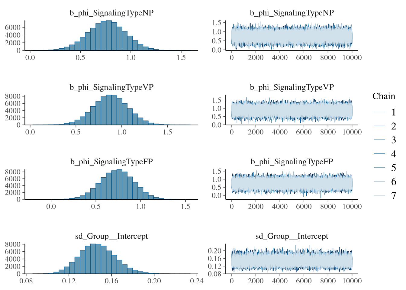
## sd(Intercept) 0.15 0.02 0.12 0.18 1.00 20154 36572
##
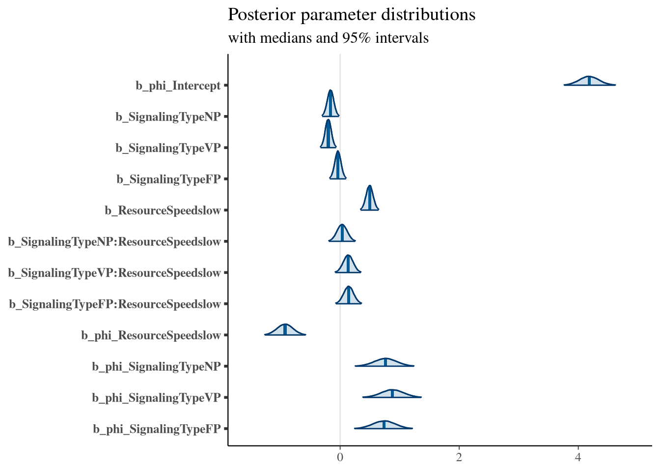
## Regression Coefficients:
## Estimate Est.Error l-95% CI u-95% CI Rhat Bulk_ESS Tail_ESS
## Intercept -0.39 0.03 -0.46 -0.33 1.00 44734 52068
## phi_Intercept 4.18 0.17 3.86 4.52 1.00 37200 45129
## SignalingTypeNP -0.16 0.05 -0.27 -0.05 1.00 29755 42816
## SignalingTypeVP -0.20 0.05 -0.30 -0.10 1.00 29152 44264
## SignalingTypeFP -0.04 0.05 -0.14 0.07 1.00 29381 43185
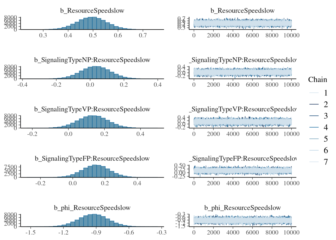
## ResourceSpeedslow 0.50 0.06 0.38 0.61 1.00 37380 48651
## SignalingTypeNP:ResourceSpeedslow 0.03 0.09 -0.14 0.20 1.00 31254 43631
## SignalingTypeVP:ResourceSpeedslow 0.14 0.08 -0.03 0.30 1.00 30461 44634
## SignalingTypeFP:ResourceSpeedslow 0.14 0.08 -0.02 0.31 1.00 30184 44332
## phi_ResourceSpeedslow -0.93 0.13 -1.19 -0.66 1.00 81743 57087
## phi_SignalingTypeNP 0.76 0.19 0.38 1.13 1.00 49050 52882
## phi_SignalingTypeVP 0.88 0.19 0.50 1.25 1.00 45817 52698
## phi_SignalingTypeFP 0.74 0.19 0.37 1.10 1.00 49874 53773
##
## Draws were sampled using sample(hmc). For each parameter, Bulk_ESS
## and Tail_ESS are effective sample size measures, and Rhat is the potential
## scale reduction factor on split chains (at convergence, Rhat = 1).Model diagnostics
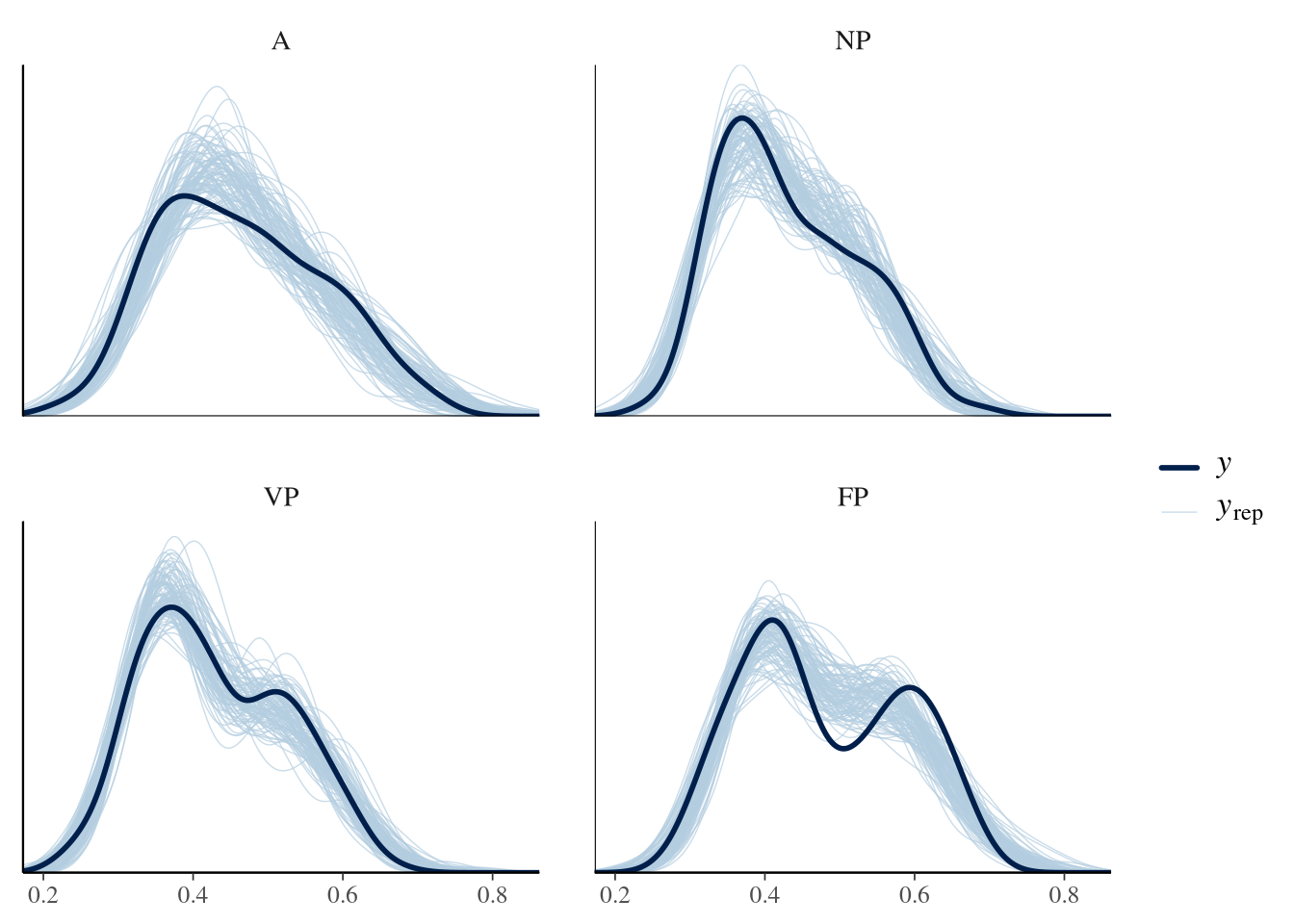
group <- m.PCR.data$SignalingType
mask <- m.PCR.data$ResourceSpeed == 'fast'

ppc_dens_overlay_grouped(m.PCR.2.y[mask],
                         m.PCR.2.yrep[1:50, mask],
                         group = group[mask])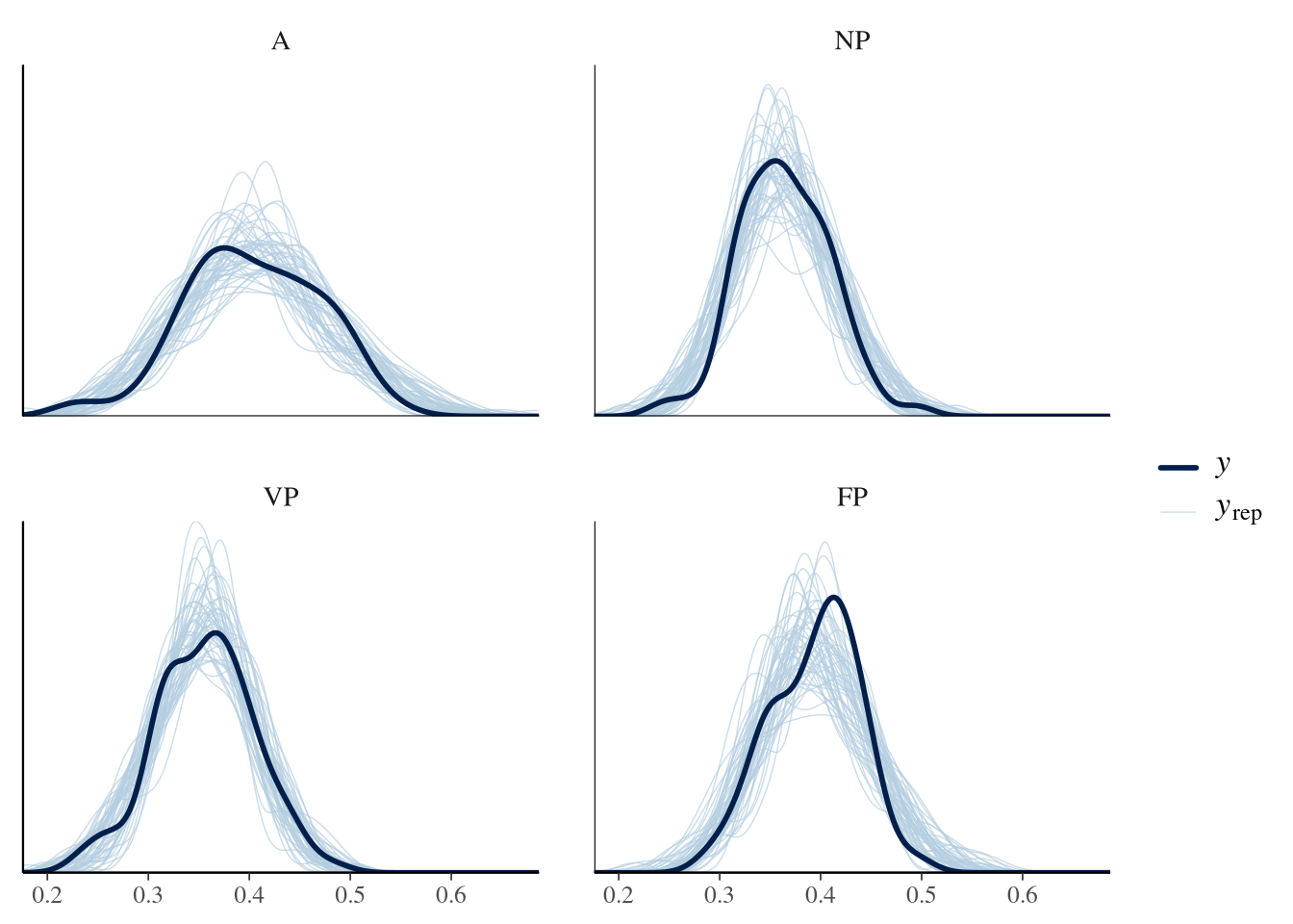
group <- m.PCR.data$SignalingType
mask <- m.PCR.data$ResourceSpeed == 'slow'

ppc_dens_overlay_grouped(m.PCR.2.y[mask],
                         m.PCR.2.yrep[1:50, mask],
                         group = group[mask])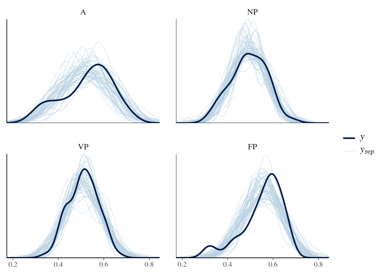
Condition comparisons
m.PCR.2.emmeans_contrast_draws.1 <- m.PCR.2.fit %>%
  emmeans(~ SignalingType * ResourceSpeed, epred = TRUE, type = "response", re_formula = m.PCR.2.formula_comparison) %>%
  contrast(method = "revpairwise", simple = "each", combine = TRUE) %>%
  gather_emmeans_draws() %>%
mutate(.value = .value * theoretical_max)m.PCR.2.comparison.1 <- m.PCR.2.emmeans_contrast_draws.1 %>%
ggdist::mean_hdci(.width = 0.9) %>%
mutate(.value = round(.value, 2), .lower = round(.lower, 2), .upper = round(.upper, 2))
m.PCR.2.comparison.1 %>%
knitr::kable("html", digits = 2) %>% kable_classic(full_width = T, position = "center", )| ResourceSpeed | SignalingType | contrast | .value | .lower | .upper | .width | .point | .interval |
|---|---|---|---|---|---|---|---|---|
| . | A | slow - fast | 4.90 | 3.95 | 5.85 | 0.9 | mean | hdci |
| . | FP | slow - fast | 6.31 | 5.34 | 7.29 | 0.9 | mean | hdci |
| . | NP | slow - fast | 5.14 | 4.12 | 6.13 | 0.9 | mean | hdci |
| . | VP | slow - fast | 6.14 | 5.19 | 7.08 | 0.9 | mean | hdci |
| fast | . | FP - A | -0.36 | -1.21 | 0.46 | 0.9 | mean | hdci |
| fast | . | FP - NP | 1.17 | 0.25 | 2.09 | 0.9 | mean | hdci |
| fast | . | FP - VP | 1.52 | 0.64 | 2.37 | 0.9 | mean | hdci |
| fast | . | NP - A | -1.53 | -2.37 | -0.68 | 0.9 | mean | hdci |
| fast | . | VP - A | -1.88 | -2.64 | -1.09 | 0.9 | mean | hdci |
| fast | . | VP - NP | -0.35 | -1.23 | 0.52 | 0.9 | mean | hdci |
| slow | . | FP - A | 1.05 | -0.02 | 2.16 | 0.9 | mean | hdci |
| slow | . | FP - NP | 2.34 | 1.25 | 3.38 | 0.9 | mean | hdci |
| slow | . | FP - VP | 1.69 | 0.63 | 2.73 | 0.9 | mean | hdci |
| slow | . | NP - A | -1.29 | -2.38 | -0.16 | 0.9 | mean | hdci |
| slow | . | VP - A | -0.64 | -1.73 | 0.46 | 0.9 | mean | hdci |
| slow | . | VP - NP | 0.65 | -0.42 | 1.72 | 0.9 | mean | hdci |
m.PCR.2.emmeans_contrast_draws.1 %>%
  filter(ResourceSpeed != '.') %>%
  rename(prediction = .value) %>%
  ggplot(
    aes(y = contrast,
        x = prediction,
        color = ResourceSpeed, shape = ResourceSpeed, fill = ResourceSpeed)) +
  facet_grid(rows = vars(ResourceSpeed)) +
  stat_pointinterval(.width = 0.9) +
  scale_color_manual(values = get_colors("Qual2", num.colors = 2, reverse = TRUE, gradient = FALSE)) +
  scale_fill_manual(values = get_colors("Qual2", num.colors = 2, reverse = TRUE, gradient = FALSE)) +
  scale_shape_manual(values = c(21, 24)) +
  labs(x = 'Prediction PCS') +
  geom_vline(aes(xintercept=0), linetype="longdash") +
  theme_nice()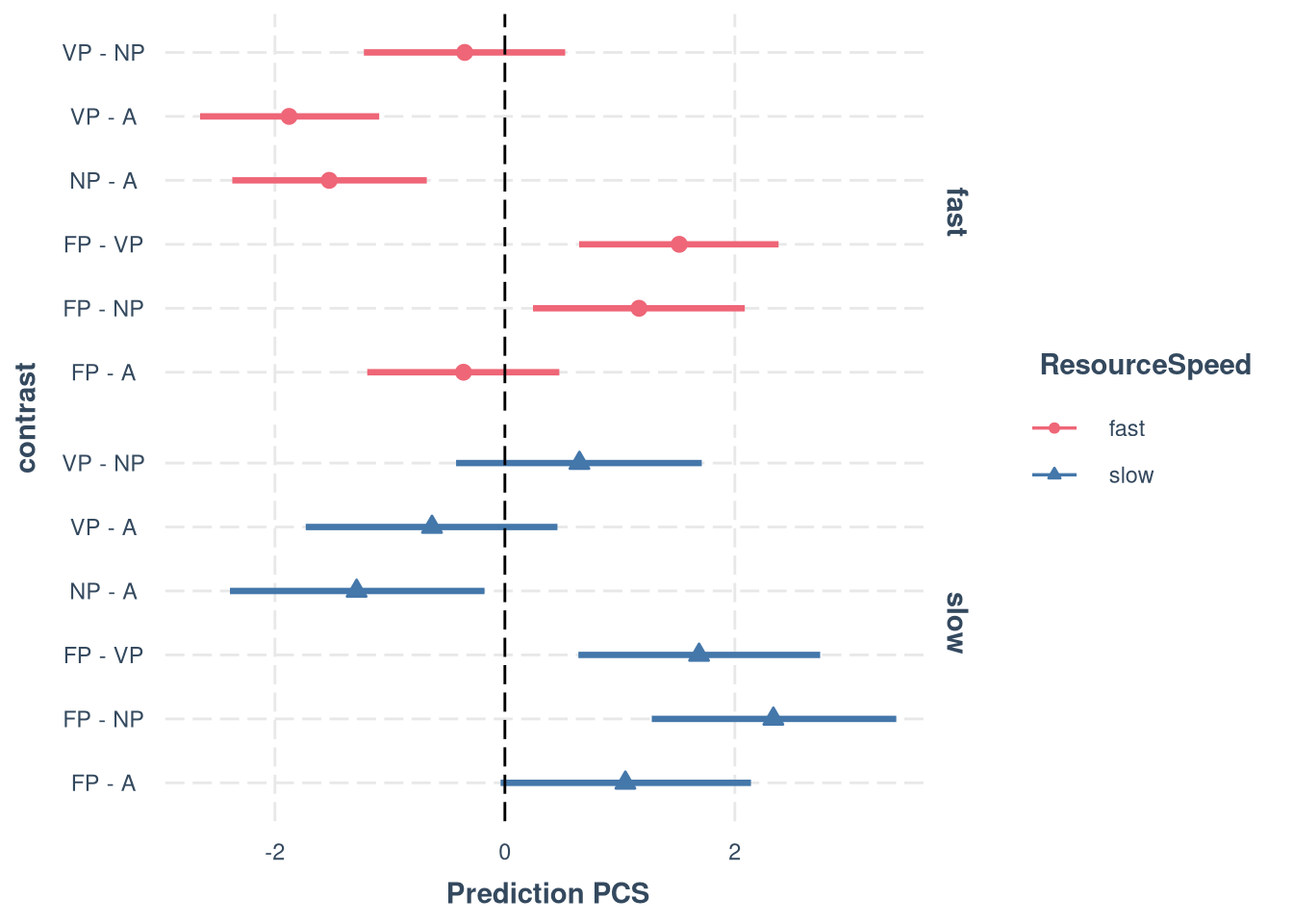
m.PCR.2.emmeans_contrast_draws.2 <- m.PCR.2.fit %>%
  emmeans(~ ResourceSpeed, epred = TRUE, type = "response", re_formula = m.PCR.2.formula_comparison) %>%
  contrast(method = "revpairwise", simple = "each", combine = TRUE) %>%
  gather_emmeans_draws() %>%
mutate(.value = .value * theoretical_max)m.PCR.2.comparison.2 <- m.PCR.2.emmeans_contrast_draws.2 %>%
ggdist::mean_hdci(.width = 0.9) %>%
mutate(.value = round(.value, 2), .lower = round(.lower, 2), .upper = round(.upper, 2))
m.PCR.2.comparison.2 %>%
knitr::kable("html", digits = 2) %>% kable_classic(full_width = T, position = "center", )| contrast | .value | .lower | .upper | .width | .point | .interval |
|---|---|---|---|---|---|---|
| slow - fast | 5.62 | 5.13 | 6.11 | 0.9 | mean | hdci |
m.PCR.2.comparison.combined_table <- bind_rows(
  m.PCR.2.comparison.2,
  m.PCR.2.comparison.1
) %>%
  select(ResourceSpeed, SignalingType, contrast, .value, .lower, .upper) %>%
  mutate(
    ResourceSpeed = ifelse(is.na(ResourceSpeed), ".", as.character(ResourceSpeed)),
    SignalingType = ifelse(is.na(SignalingType), ".", as.character(SignalingType)),
    sig = (.lower * .upper) > 0,
    Estimate = sprintf("%.2f", .value),
    Estimate = ifelse(sig, paste0("\\textbf{", Estimate, "}"), Estimate),
    hpdi = sprintf("[%.2f, %.2f]", .lower, .upper),
    hpdi = ifelse(sig, paste0("\\textbf{", hpdi, "}"), hpdi)
  ) %>%
  select(ResourceSpeed, SignalingType, contrast, Estimate, hpdi)

# (Optional) Rename columns for publication
colnames(m.PCR.2.comparison.combined_table) <- c(
  "Resource Speed", "Payoff Condition", "Contrast", "Mean", "90\\% HPDI"
)


kbl <- kable(
  m.PCR.2.comparison.combined_table,
  format = "latex",
  booktabs = TRUE,
  align = c("l", "l", "l", "r", "r"),
  caption = "Posterior Estimates Point Collection Rate",
  escape = FALSE
  ) %>%
    kable_styling(latex_options = "hold_position") %>%
    row_spec(0, bold = TRUE)

unique_speeds <- unique(m.PCR.2.comparison.combined_table$`Resource Speed`)
start <- 1
for (speed in unique_speeds) {
  n_rows <- sum(m.PCR.2.comparison.combined_table$`Resource Speed` == speed)
  if (speed != ".") {
    kbl <- group_rows(kbl, speed, start, start + n_rows - 1)
  }
  start <- start + n_rows
}

writeLines(kbl, paste0(comparisons, "pcr_2_comparison_combined.tex"))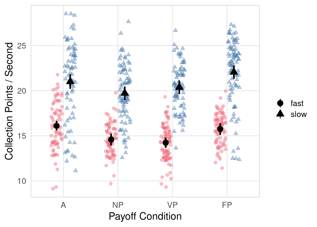
Model Comparison
m.PCR.1.loo_model <- loo(m.PCR.1.fit, moment_match = F, reloo = F, draws = 1000)
m.PCR.2.loo_model <- loo(m.PCR.2.fit, moment_match = F, reloo = F, draws = 1000)##
## Computed from 70000 by 621 log-likelihood matrix.
##
## Estimate SE
## elpd_loo 616.5 6.5
## p_loo 3.6 0.2
## looic -1233.0 13.1
## ------
## MCSE of elpd_loo is 0.0.
## MCSE and ESS estimates assume MCMC draws (r_eff in [0.9, 1.8]).
##
## All Pareto k estimates are good (k < 0.7).
## See help('pareto-k-diagnostic') for details.##
## Computed from 70000 by 621 log-likelihood matrix.
##
## Estimate SE
## elpd_loo 847.9 21.2
## p_loo 102.0 6.4
## looic -1695.8 42.4
## ------
## MCSE of elpd_loo is NA.
## MCSE and ESS estimates assume MCMC draws (r_eff in [0.4, 2.2]).
##
## Pareto k diagnostic values:
## Count Pct. Min. ESS
## (-Inf, 0.7] (good) 619 99.7% 2202
## (0.7, 1] (bad) 2 0.3% <NA>
## (1, Inf) (very bad) 0 0.0% <NA>
## See help('pareto-k-diagnostic') for details.## elpd_diff se_diff elpd_loo se_elpd_loo p_loo se_p_loo looic se_looic
## m.PCR.2.fit 0.000 0.000 847.922 21.207 101.963 6.445 -1695.844 42.414
## m.PCR.1.fit -231.435 16.536 616.487 6.544 3.584 0.235 -1232.974 13.088