Static Connecitvity

m.StaticConnectivity.data <- time_series_data %>%
  filter(SignalingType != 'A') %>%
  mutate(SignalingType = factor(SignalingType, levels = c('NP', 'VP', 'FP'))) %>%
  select(Participant, SignalingType, ResourceSpeed, Time, State, InDegree, OutDegree)

head(m.StaticConnectivity.data)

In-degree model

m.StaticConnectivity.Indegree.formula <- brmsformula(
  InDegree ~ ResourceSpeed * SignalingType + (1 | Participant),
  family = poisson()
  )

m.StaticConnectivity.Indegree.formula_comparison <- brmsformula(
  InDegree ~ ResourceSpeed * SignalingType,
  family = poisson()
  )

m.StaticConnectivity.Indegree.priors <- c(
    prior(normal(0, 1), class = b),
    prior(normal(0, 1), class = Intercept),
    prior(normal(0, 0.1), class = sd, lb = 0)
    # prior(exponential(0.01), class = phi, lb = 0)
)

Prior predictive checks

m.StaticConnectivity.Indegree.fit_prior <- brm(
  formula = m.StaticConnectivity.Indegree.formula,
  data    = m.StaticConnectivity.data,
  prior   = m.StaticConnectivity.Indegree.priors,
  chains  = 4,
  cores   = 4,
  seed    = 42,
  iter    = 2000,
  file = paste0(fits_path, 'static_connectivity_in_degree_1_prior.rds'),
  sample_prior = "only",
  backend = "cmdstanr",
  threads = threading(100),
  control = list(adapt_delta = 0.95),
  save_pars = save_pars(all = TRUE))

plot(conditional_effects(m.StaticConnectivity.Indegree.fit_prior, 
                         ndraws = 20, spaghetti = TRUE), points = F, ask = F)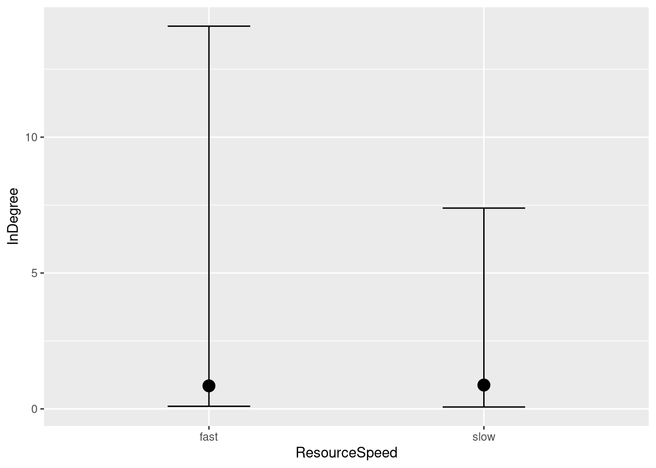

Model fitting

m.StaticConnectivity.Indegree.fit <- brm(
  formula = m.StaticConnectivity.Indegree.formula,
  data    = m.StaticConnectivity.data,
  prior   = m.StaticConnectivity.Indegree.priors,
  chains  = 4,
  cores   = 4,
  seed    = 42,
  warmup  = 500,
  iter    = 2000,
  file = paste0(fits_path, 'static_connectivity_in_degree_1.rds'),
  backend = "cmdstanr",
  threads = threading(100),
  control = list(adapt_delta = 0.95),
  save_pars = save_pars(all = TRUE))

summary(m.StaticConnectivity.Indegree.fit)

##  Family: poisson 
##   Links: mu = log 
## Formula: InDegree ~ ResourceSpeed * SignalingType + (1 | Participant) 
##    Data: m.StaticConnectivity.data (Number of observations: 410697) 
##   Draws: 4 chains, each with iter = 2000; warmup = 500; thin = 1;
##          total post-warmup draws = 6000
## 
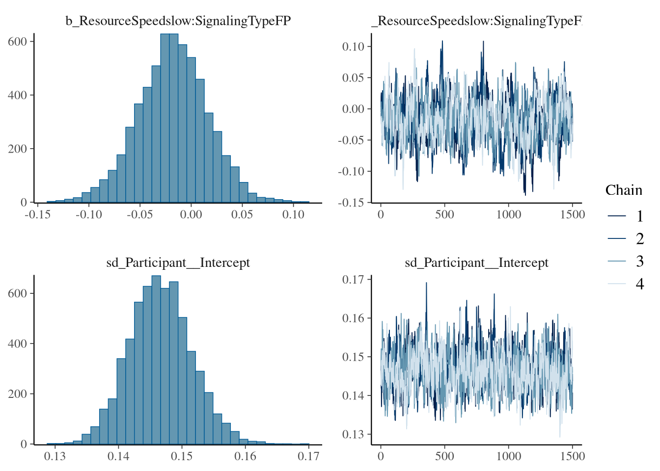
## Multilevel Hyperparameters:
## ~Participant (Number of levels: 477) 
##               Estimate Est.Error l-95% CI u-95% CI Rhat Bulk_ESS Tail_ESS
## sd(Intercept)     0.15      0.00     0.14     0.16 1.00      717     1410
## 
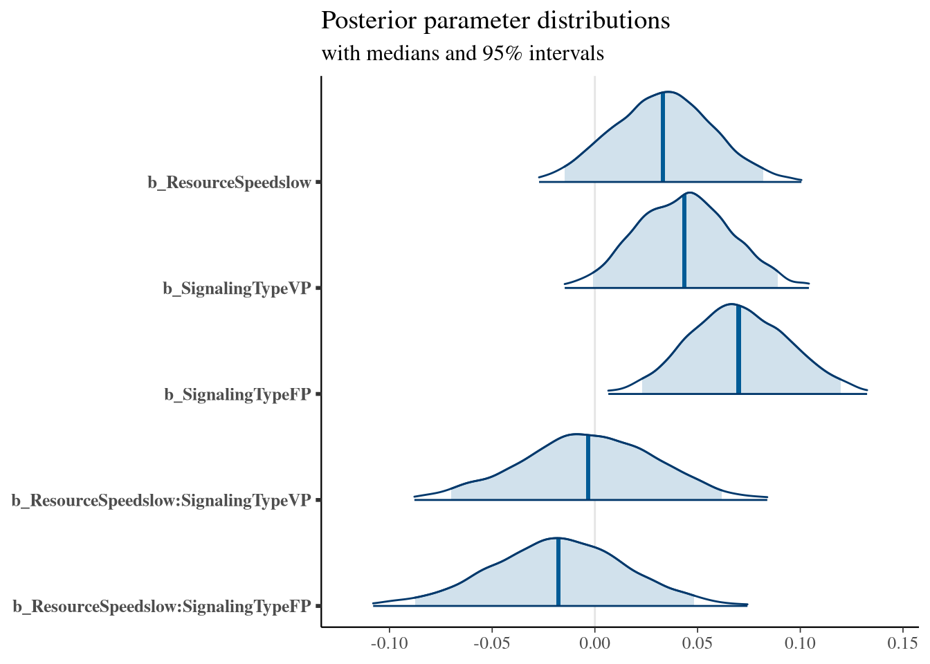
## Regression Coefficients:
##                                   Estimate Est.Error l-95% CI u-95% CI Rhat Bulk_ESS Tail_ESS
## Intercept                             0.04      0.02     0.00     0.07 1.01      316      631
## ResourceSpeedslow                     0.03      0.02    -0.01     0.08 1.01      314      543
## SignalingTypeVP                       0.04      0.02    -0.00     0.09 1.01      334      846
## SignalingTypeFP                       0.07      0.02     0.02     0.12 1.01      298      712
## ResourceSpeedslow:SignalingTypeVP    -0.00      0.03    -0.07     0.06 1.01      315      883
## ResourceSpeedslow:SignalingTypeFP    -0.02      0.03    -0.09     0.05 1.00      272      489
## 
## Draws were sampled using sample(hmc). For each parameter, Bulk_ESS
## and Tail_ESS are effective sample size measures, and Rhat is the potential
## scale reduction factor on split chains (at convergence, Rhat = 1).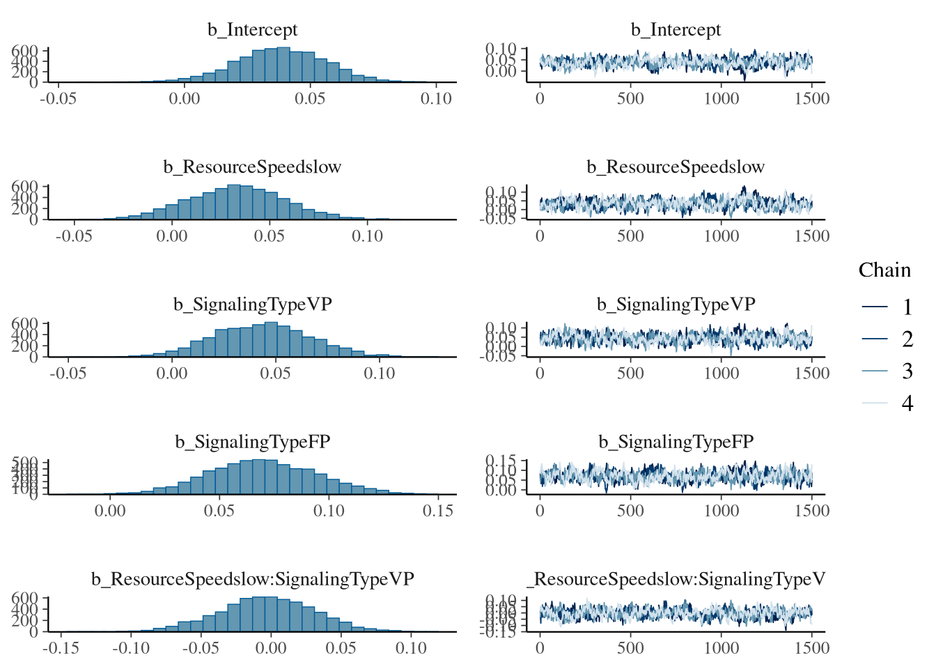

Model diagnostics

plot(m.StaticConnectivity.Indegree.fit, ask = F)

Model predictions

Condition comparisons

plot(conditional_effects(m.StaticConnectivity.Indegree.fit), points = F, ask = F)

m.StaticConnectivity.Indegree.emmeans_contrast_draws <- m.StaticConnectivity.Indegree.fit %>%
  emmeans(~ SignalingType * ResourceSpeed, 
          epred = TRUE, 
          type = "response",
          re_formula = m.StaticConnectivity.Indegree.formula_comparison
         ) %>%
  contrast(method = "revpairwise", simple = "each", combine = TRUE) %>%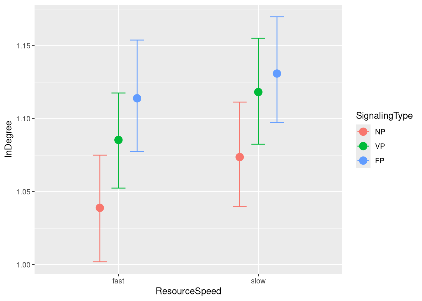 
  gather_emmeans_draws()

ResourceSpeed	SignalingType	contrast	.value	.lower	.upper	.width	.point	.interval
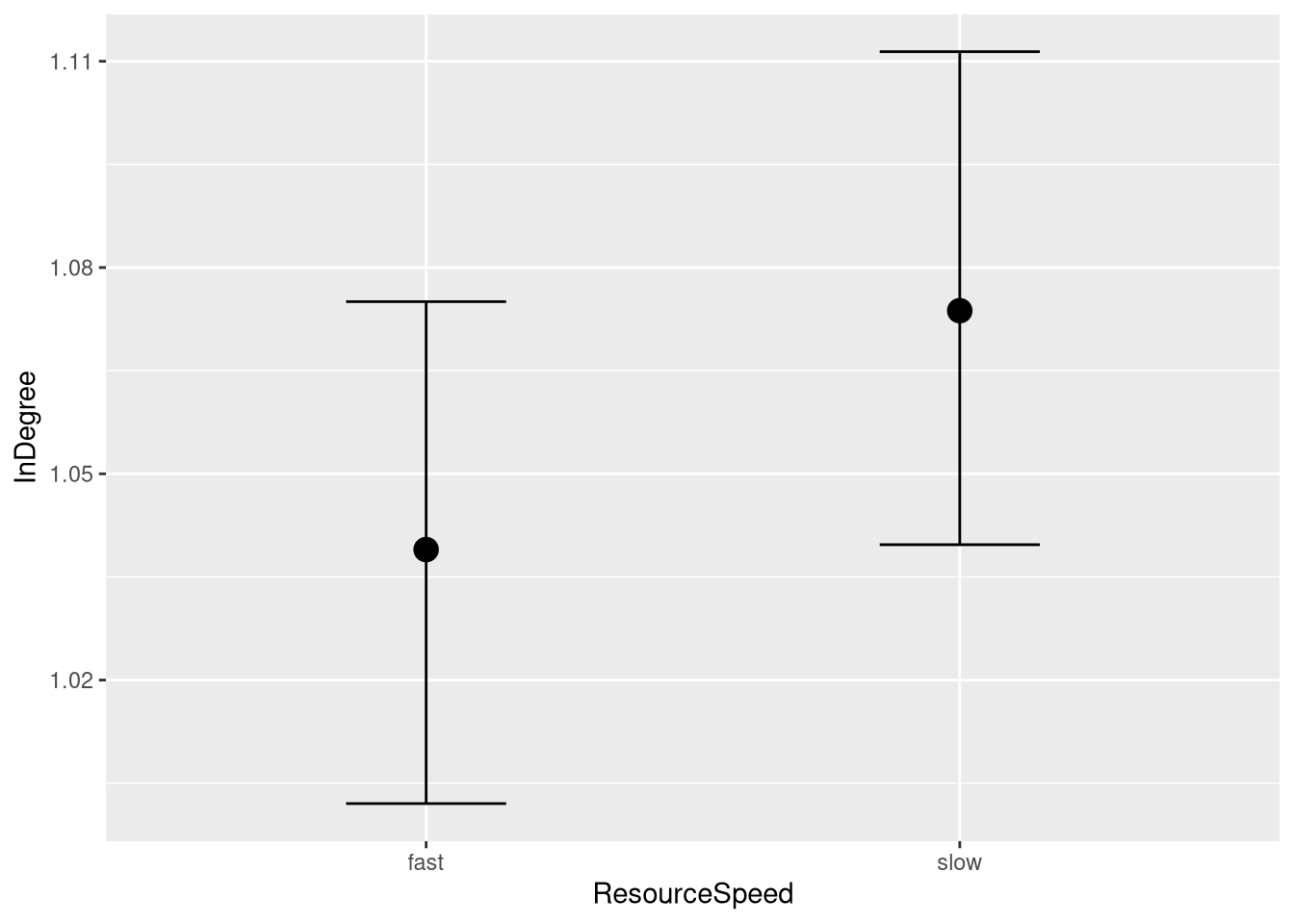
.	FP	slow - fast	0.02	-0.03	0.06	0.9	mean	hdci
.	NP	slow - fast	0.04	-0.01	0.08	0.9	mean	hdci
.	VP	slow - fast	0.03	-0.01	0.07	0.9	mean	hdci
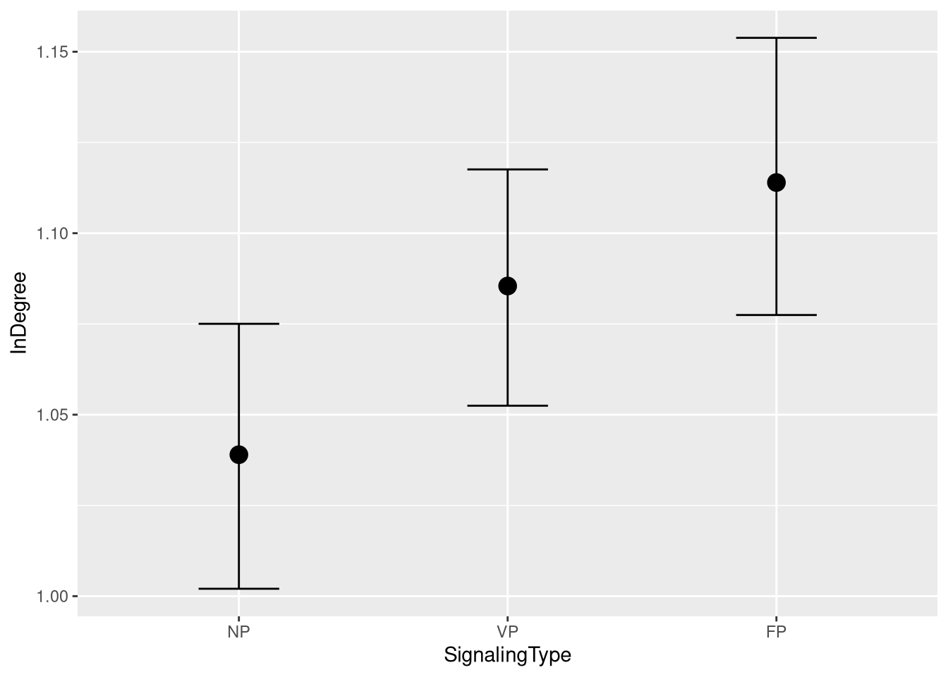
fast	.	FP - NP	0.08	0.03	0.12	0.9	mean	hdci
fast	.	FP - VP	0.03	-0.02	0.07	0.9	mean	hdci
fast	.	VP - NP	0.05	0.01	0.09	0.9	mean	hdci
slow	.	FP - NP	0.06	0.01	0.10	0.9	mean	hdci
slow	.	FP - VP	0.01	-0.03	0.06	0.9	mean	hdci
slow	.	VP - NP	0.04	0.00	0.09	0.9	mean	hdci

m.StaticConnectivity.Indegree.comparison.combined_table <- m.StaticConnectivity.Indegree.comparison %>%
  select(ResourceSpeed, SignalingType, contrast, .value, .lower, .upper) %>%
  mutate(
    ResourceSpeed = ifelse(is.na(ResourceSpeed), ".", as.character(ResourceSpeed)),
    SignalingType = ifelse(is.na(SignalingType), ".", as.character(SignalingType)),
    sig = (.lower * .upper) > 0,
    Estimate = sprintf("%.2f", .value),
    Estimate = ifelse(sig, paste0("\\textbf{", Estimate, "}"), Estimate),
    hpdi = sprintf("[%.2f, %.2f]", .lower, .upper),
    hpdi = ifelse(sig, paste0("\\textbf{", hpdi, "}"), hpdi)
  ) %>%
  select(ResourceSpeed, SignalingType, contrast, Estimate, hpdi)

colnames(m.StaticConnectivity.Indegree.comparison.combined_table) <- c(
  "Resource Speed", "Payoff Condition", "Contrast", "Mean", "90\\% HPDI"
)

kbl <- kable(
  m.StaticConnectivity.Indegree.comparison.combined_table,
  format = "latex",
  booktabs = TRUE,
  align = c("l", "l", "l", "r", "r"),
  caption = "Posterior Estimates In Degree",
  escape = FALSE
  ) %>% 
    kable_styling(latex_options = "hold_position") %>%
    row_spec(0, bold = TRUE)

unique_speeds <- unique(m.StaticConnectivity.Indegree.comparison.combined_table$`Resource Speed`)
start <- 1
for (speed in unique_speeds) {
  n_rows <- sum(m.StaticConnectivity.Indegree.comparison.combined_table$`Resource Speed` == speed)
  if (speed != ".") { 
    kbl <- group_rows(kbl, speed, start, start + n_rows - 1)
  }
  start <- start + n_rows
}

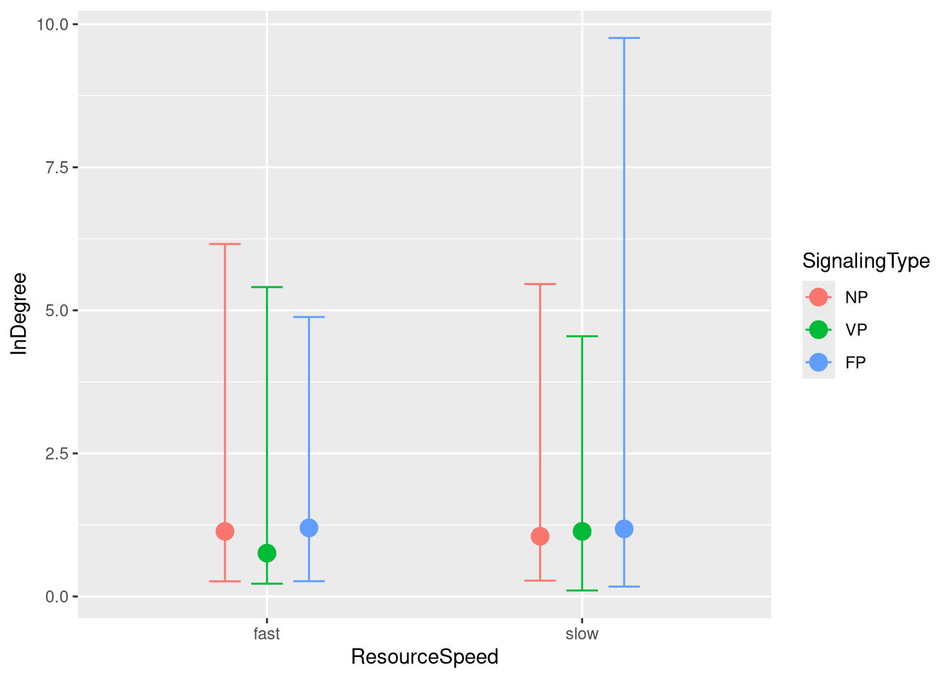
writeLines(kbl, paste0(comparisons, "static_connectiveity_in_degree_comparison.tex"))

Figure

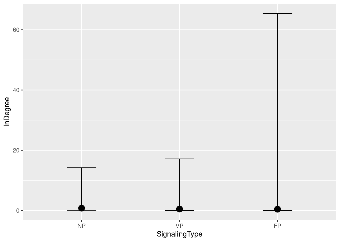
static_connectivity_in_degree_fig <- m.StaticConnectivity.data %>% 
  data_grid(ResourceSpeed, SignalingType) %>%
  tidybayes::add_epred_draws(m.StaticConnectivity.Indegree.fit, 
                             allow_new_levels = TRUE, 
                             re_formula = m.StaticConnectivity.Indegree.formula_comparison) %>%
  ggplot(aes(x = SignalingType, 
             y = .epred, 
             color = SignalingType,
             fill = SignalingType,
             shape = ResourceSpeed)) +
  ggdist::stat_pointinterval(
    position = position_dodge(width = .5),
    point_interval = "mean_qi",
    .width = 0.9, # c(0.5, 0.9),
    point_size = 3.6,
    ) +
  scale_color_manual(values = c("#DF536B", "#61D04F", "#2297E6"), guide = guide_legend(title = "Signaling")) +
  scale_fill_manual(values = c("#DF536B", "#61D04F", "#2297E6"), guide = guide_legend(title = "Signaling")) +
  scale_shape_manual(values = c(21, 24), guide = guide_legend(title = "Resource")) +
  theme_clean() +
  panel_border() +
  theme(legend.position    = "none") +
  labs(x = '', 
       y = 'In Degree')
  
static_connectivity_in_degree_fig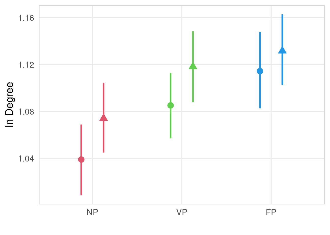

Out-degree model

m.StaticConnectivity.Outdegree.formula <- brmsformula(
  OutDegree ~ ResourceSpeed * SignalingType + (1 | Participant),
  family = poisson()
  )

m.StaticConnectivity.Outdegree.formula_comparison <- brmsformula(
  OutDegree ~ ResourceSpeed * SignalingType,
  family = poisson()
  )

m.StaticConnectivity.Outdegree.priors <- c(
    prior(normal(0, 1), class = b),
    prior(normal(0, 1), class = Intercept),
    prior(normal(0, 0.1), class = sd, lb = 0)
    # prior(exponential(0.01), class = phi, lb = 0)
)

Prior predictive checks

m.StaticConnectivity.Outdegree.fit_prior <- brm(
  formula = m.StaticConnectivity.Outdegree.formula,
  data    = m.StaticConnectivity.data,
  prior   = m.StaticConnectivity.Outdegree.priors,
  chains  = 4,
  cores   = 4,
  seed    = 42,
  iter    = 2000,
  file = paste0(fits_path, 'static_connectivity_out_degree_1_prior.rds'),
  sample_prior = "only",
  backend = "cmdstanr",
  threads = threading(100),
  control = list(adapt_delta = 0.95),
  save_pars = save_pars(all = TRUE))

plot(conditional_effects(m.StaticConnectivity.Outdegree.fit_prior, 
                         ndraws = 20, spaghetti = TRUE), points = F, ask = F)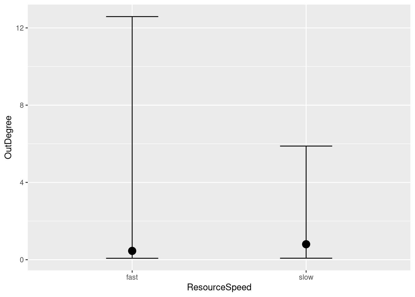

Model fitting

m.StaticConnectivity.Outdegree.fit <- brm(
  formula = m.StaticConnectivity.Outdegree.formula,
  data    = m.StaticConnectivity.data,
  prior   = m.StaticConnectivity.Outdegree.priors,
  chains  = 4,
  cores   = 4,
  seed    = 42,
  warmup  = 500,
  iter    = 2000,
  file = paste0(fits_path, 'static_connectivity_out_degree_1.rds'),
  backend = "cmdstanr",
  threads = threading(100),
  control = list(adapt_delta = 0.95),
  save_pars = save_pars(all = TRUE))

summary(m.StaticConnectivity.Outdegree.fit)

##  Family: poisson 
##   Links: mu = log 
## Formula: OutDegree ~ ResourceSpeed * SignalingType + (1 | Participant) 
##    Data: m.StaticConnectivity.data (Number of observations: 410697) 
##   Draws: 4 chains, each with iter = 2000; warmup = 500; thin = 1;
##          total post-warmup draws = 6000
## 
## Multilevel Hyperparameters:
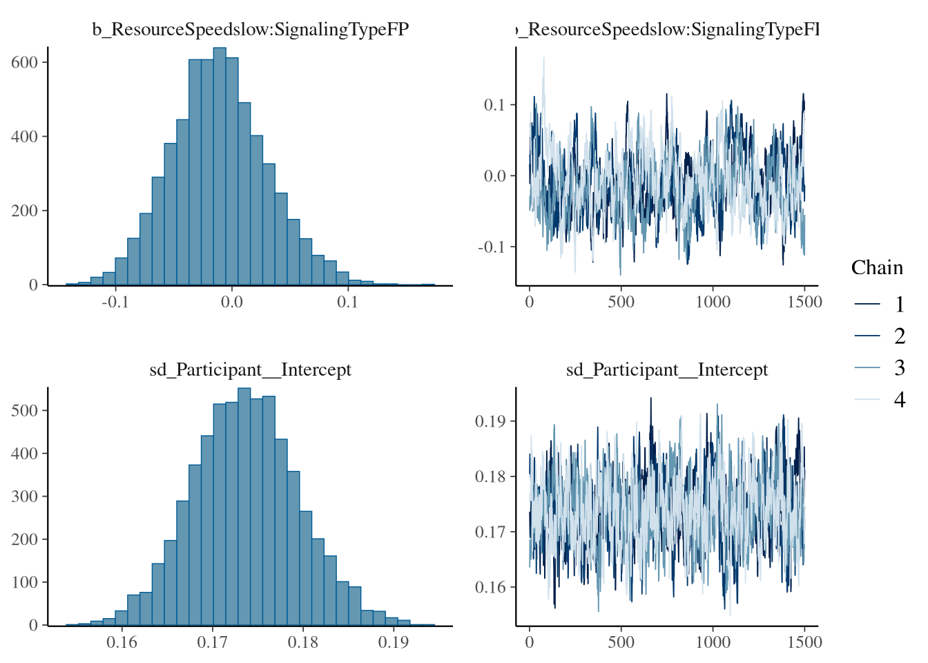
## ~Participant (Number of levels: 477) 
##               Estimate Est.Error l-95% CI u-95% CI Rhat Bulk_ESS Tail_ESS
## sd(Intercept)     0.17      0.01     0.16     0.19 1.00      519      985
## 
## Regression Coefficients:
##                                   Estimate Est.Error l-95% CI u-95% CI Rhat Bulk_ESS Tail_ESS
## Intercept                             0.02      0.02    -0.02     0.06 1.01      289      691
## ResourceSpeedslow                     0.02      0.03    -0.03     0.08 1.01      287      639
## SignalingTypeVP                       0.03      0.03    -0.02     0.09 1.01      241      450
## SignalingTypeFP                       0.07      0.03     0.01     0.13 1.01      241      547
## ResourceSpeedslow:SignalingTypeVP    -0.01      0.04    -0.08     0.08 1.01      229      394
## ResourceSpeedslow:SignalingTypeFP    -0.01      0.04    -0.09     0.08 1.02      245      573
## 
## Draws were sampled using sample(hmc). For each parameter, Bulk_ESS
## and Tail_ESS are effective sample size measures, and Rhat is the potential
## scale reduction factor on split chains (at convergence, Rhat = 1).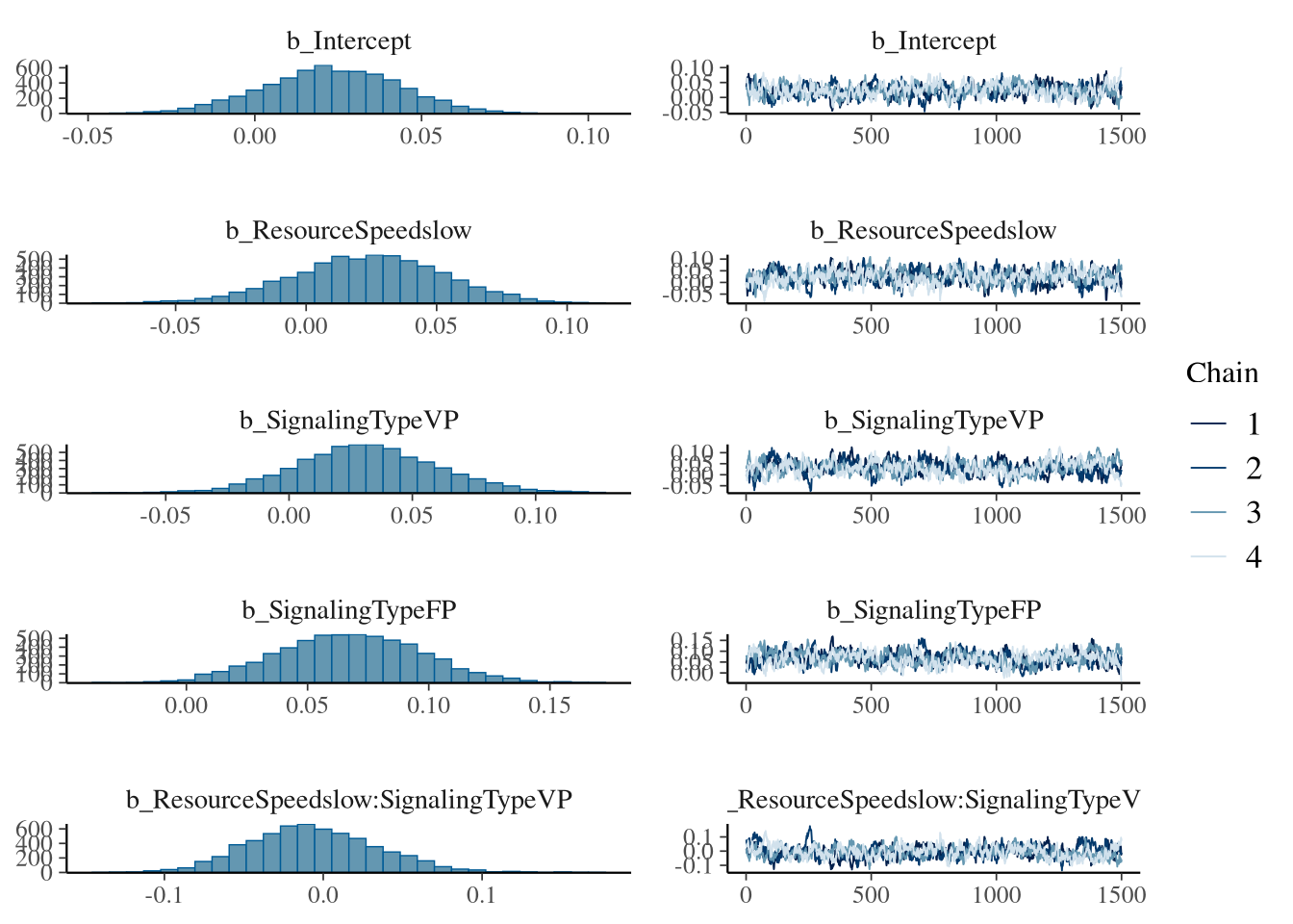

Model diagnostics

plot(m.StaticConnectivity.Outdegree.fit, ask = F)

Model predictions

Condition comparisons

plot(conditional_effects(m.StaticConnectivity.Outdegree.fit), points = F, ask = F)

m.StaticConnectivity.Outdegree.emmeans_contrast_draws <- m.StaticConnectivity.Outdegree.fit %>%
  emmeans(~ SignalingType * ResourceSpeed, 
          epred = TRUE, 
          type = "response",
          re_formula = m.StaticConnectivity.Outdegree.formula_comparison
         ) %>%
  contrast(method = "revpairwise", simple = "each", combine = TRUE) %>%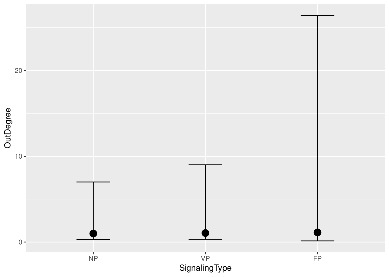 
  gather_emmeans_draws()

ResourceSpeed	SignalingType	contrast	.value	.lower	.upper	.width	.point	.interval
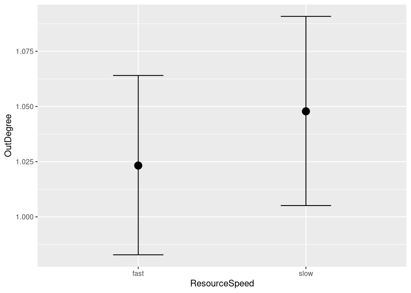
.	FP	slow - fast	0.01	-0.04	0.06	0.9	mean	hdci
.	NP	slow - fast	0.02	-0.03	0.07	0.9	mean	hdci
.	VP	slow - fast	0.02	-0.03	0.07	0.9	mean	hdci
fast	.	FP - NP	0.07	0.02	0.12	0.9	mean	hdci
fast	.	FP - VP	0.04	-0.01	0.09	0.9	mean	hdci
fast	.	VP - NP	0.03	-0.02	0.08	0.9	mean	hdci
slow	.	FP - NP	0.06	0.01	0.11	0.9	mean	hdci
slow	.	FP - VP	0.03	-0.02	0.08	0.9	mean	hdci
slow	.	VP - NP	0.03	-0.02	0.08	0.9	mean	hdci

m.StaticConnectivity.Outdegree.comparison.combined_table <- m.StaticConnectivity.Outdegree.comparison %>%
  select(ResourceSpeed, SignalingType, contrast, .value, .lower, .upper) %>%
  mutate(
    ResourceSpeed = ifelse(is.na(ResourceSpeed), ".", as.character(ResourceSpeed)),
    SignalingType = ifelse(is.na(SignalingType), ".", as.character(SignalingType)),
    sig = (.lower * .upper) > 0,
    Estimate = sprintf("%.2f", .value),
    Estimate = ifelse(sig, paste0("\\textbf{", Estimate, "}"), Estimate),
    hpdi = sprintf("[%.2f, %.2f]", .lower, .upper),
    hpdi = ifelse(sig, paste0("\\textbf{", hpdi, "}"), hpdi)
  ) %>%
  select(ResourceSpeed, SignalingType, contrast, Estimate, hpdi)

colnames(m.StaticConnectivity.Outdegree.comparison.combined_table) <- c(
  "Resource Speed", "Payoff Condition", "Contrast", "Mean", "90\\% HPDI"
)

kbl <- kable(
  m.StaticConnectivity.Outdegree.comparison.combined_table,
  format = "latex",
  booktabs = TRUE,
  align = c("l", "l", "l", "r", "r"),
  caption = "Posterior Estimates Out Degree",
  escape = FALSE
  ) %>% 
    kable_styling(latex_options = "hold_position") %>%
    row_spec(0, bold = TRUE)

unique_speeds <- unique(m.StaticConnectivity.Outdegree.comparison.combined_table$`Resource Speed`)
start <- 1
for (speed in unique_speeds) {
  n_rows <- sum(m.StaticConnectivity.Outdegree.comparison.combined_table$`Resource Speed` == speed)
  if (speed != ".") { 
    kbl <- group_rows(kbl, speed, start, start + n_rows - 1)
  }
  start <- start + n_rows
}

writeLines(kbl, paste0(comparisons, "static_connectiveity_out_degree_comparison.tex"))

Figure

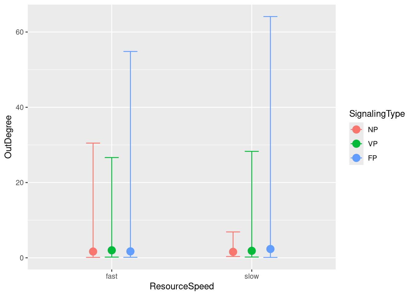
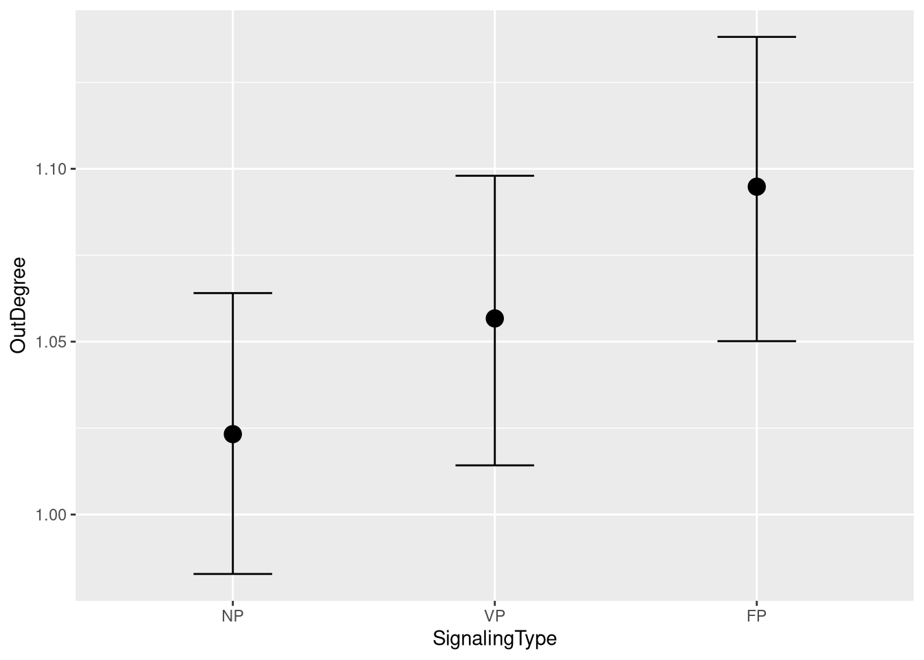
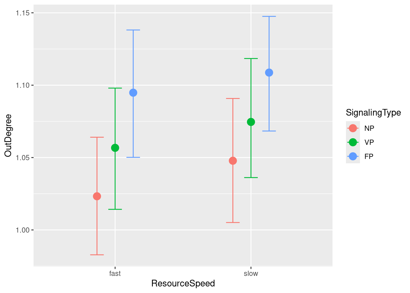
static_connectivity_out_degree_fig <- m.StaticConnectivity.data %>% 
  data_grid(ResourceSpeed, SignalingType) %>%
  tidybayes::add_epred_draws(m.StaticConnectivity.Outdegree.fit, 
                             allow_new_levels = TRUE, 
                             re_formula = m.StaticConnectivity.Outdegree.formula_comparison) %>%
  ggplot(aes(x = SignalingType, 
             y = .epred, 
             color = SignalingType,
             fill = SignalingType,
             shape = ResourceSpeed)) +
  ggdist::stat_pointinterval(
    position = position_dodge(width = .5),
    point_interval = "mean_qi",
    .width = 0.9, # c(0.5, 0.9),
    point_size = 3.6,
    ) +
  scale_color_manual(values = c("#DF536B", "#61D04F", "#2297E6"), guide = guide_legend(title = "Signaling")) +
  scale_fill_manual(values = c("#DF536B", "#61D04F", "#2297E6"), guide = guide_legend(title = "Signaling")) +
  scale_shape_manual(values = c(21, 24), guide = guide_legend(title = "Resource")) +
  theme_clean() +
  theme(legend.position    = "none") + # "bottom"
  panel_border() +
  labs(x = '',
       y = 'Out Degree')
  
static_connectivity_out_degree_fig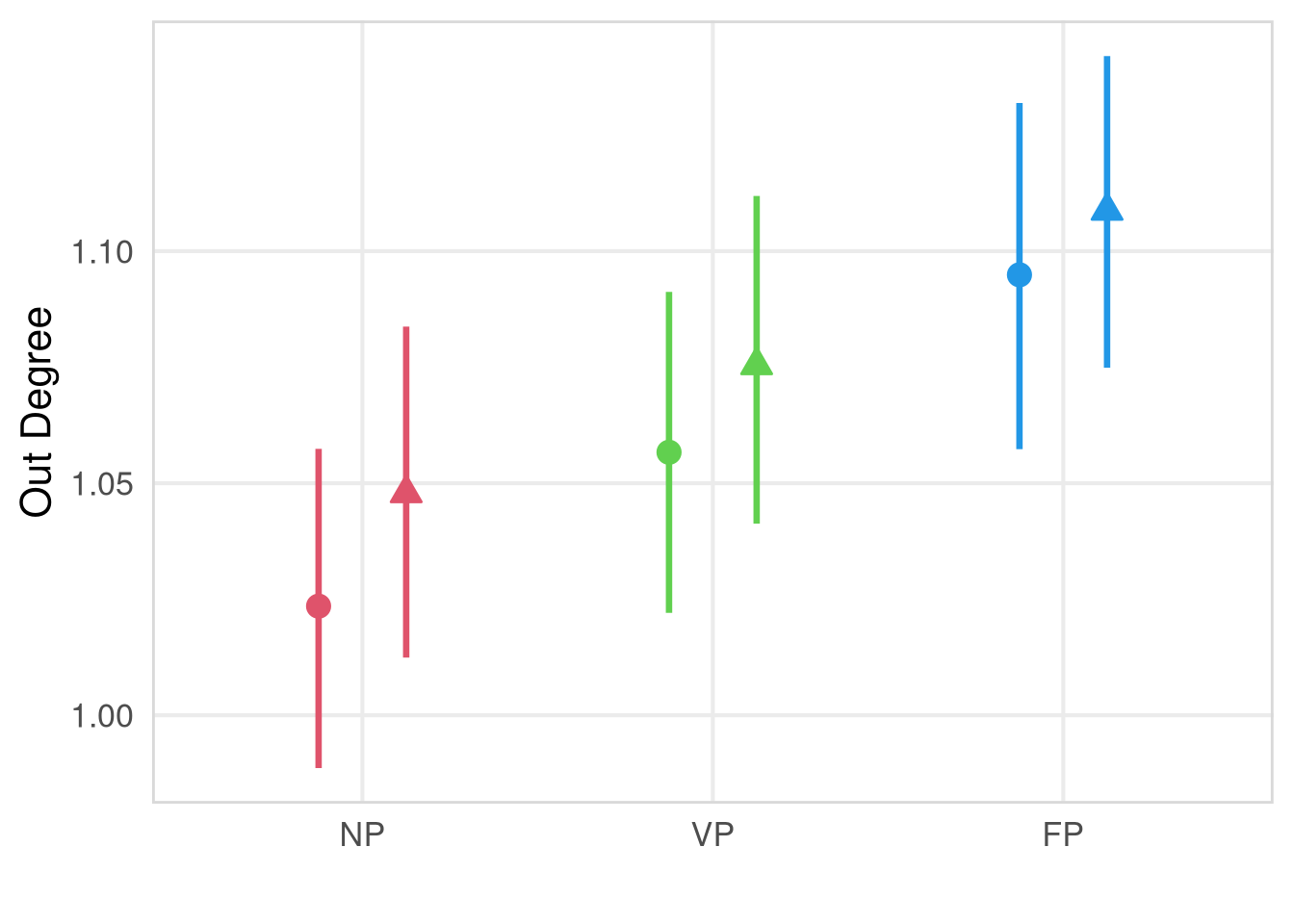

Correlation

degree_corr_fig <- m.StaticConnectivity.data %>% 
  group_by(Participant, ResourceSpeed, SignalingType) %>% 
  summarise(InDegree = mean(InDegree), OutDegree = mean(OutDegree)) %>% 
  ggplot(aes(x = InDegree, y = OutDegree, color = SignalingType)) +
  geom_point() +
  # geom_smooth(method = "lm", se = FALSE, aes(group = SignalingType, color = SignalingType)) +
  facet_grid(cols = vars(ResourceSpeed)) +
  scale_color_manual(values = c("#DF536B", "#61D04F", "#2297E6"), guide = guide_legend(title = "Payoff Condition")) +
  scale_fill_manual(values = c("#DF536B", "#61D04F", "#2297E6"), guide = guide_legend(title = "Payoff Condition")) +
  theme_clean() +
  theme(legend.position    = "bottom") +
  panel_border() +
  labs(x = 'In Degree', 
       y = 'Out Degree') +
  # stat_cor(aes(label = paste(..r.label.., ..p.label.., sep = "~`,`~")), 
  #          method = "pearson", label.x.npc = "middle", label.y.npc = "top", size = 3)
  stat_cor(aes(label = paste(..r.label.., ifelse(..p.value.. < 0.001, "p < 0.001", ..p.label..), sep = "~`,`~")), 
         method = "pearson", label.x.npc = "middle", label.y.npc = "top", size = 3, show.legend = FALSE)
degree_corr_fig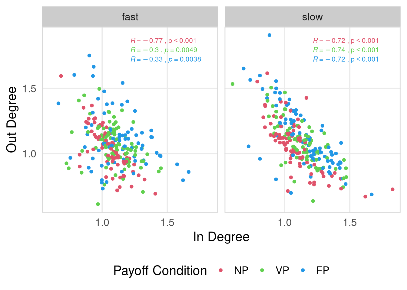

m.StaticConnectivity.data %>% 
  group_by(Participant, ResourceSpeed, SignalingType) %>% 
  summarise(InDegree = mean(InDegree), OutDegree = mean(OutDegree), .groups = "drop") %>%
  ungroup() %>% 
  do(tidy(cor.test(.$InDegree, .$OutDegree, method = "pearson")))