Resouece Discoveries
resource_discoveries_data %>%
  group_by(ResourceSpeed) %>%
  summarise(NumberOfUniqueEvents = n_distinct(Event)) %>%
  arrange(ResourceSpeed)
n_resource_discovery_event <- resource_discoveries_data %>%
group_by(SignalingType, ResourceSpeed) %>%
summarise(NumberOfUniqueEvents = n_distinct(Event)) %>%
arrange(ResourceSpeed, SignalingType)
n_resource_discovery_event %>%
knitr::kable("html", digits = 2) %>% kable_classic(full_width = T, position = "center", )| SignalingType | ResourceSpeed | NumberOfUniqueEvents |
|---|---|---|
| A | fast | 383 |
| NP | fast | 126 |
| VP | fast | 173 |
| FP | fast | 147 |
| A | slow | 212 |
| NP | slow | 17 |
| VP | slow | 21 |
| FP | slow | 11 |
writeLines(kable(n_resource_discovery_event, format = "latex"),
           paste0(comparisons, "n_resource_discovery_event_table.tex"))
resource_discoveries_data %>%
filter(str_starts(Event, "NS-18")) %>%
summarise(NumberOfUniqueEvents = n_distinct(Event))resource_discoveries_data_vp %>%
group_by(ResourceSpeed, SignalingType) %>%
summarise(UniqueEvents = n_distinct(Event)) %>%
arrange(ResourceSpeed, SignalingType) %>%
knitr::kable("html", digits = 2) %>% kable_classic(full_width = T, position = "center", )| ResourceSpeed | SignalingType | UniqueEvents |
|---|---|---|
| fast | VP_NS | 107 |
| fast | VP_S | 66 |
| slow | VP_NS | 9 |
| slow | VP_S | 12 |
resource_discoveries_data_vp %>%
  mutate(Group = str_extract(Event, "^[^-_]+[-_][0-9]+")) %>%
  group_by(ResourceSpeed, SignalingType, Group) %>%
  summarise(UniqueEvents = n_distinct(Event)) %>%
  arrange(ResourceSpeed, Group, SignalingType) %>%
knitr::kable("html", digits = 2) %>% kable_classic(full_width = T, position = "center", )| ResourceSpeed | SignalingType | Group | UniqueEvents |
|---|---|---|---|
| fast | VP_NS | VP-10 | 12 |
| fast | VP_S | VP-10 | 1 |
| fast | VP_NS | VP-13 | 4 |
| fast | VP_S | VP-13 | 6 |
| fast | VP_NS | VP-14 | 1 |
| fast | VP_S | VP-14 | 6 |
| fast | VP_NS | VP-15 | 6 |
| fast | VP_S | VP-15 | 2 |
| fast | VP_NS | VP-16 | 11 |
| fast | VP_S | VP-16 | 1 |
| fast | VP_NS | VP-19 | 1 |
| fast | VP_S | VP-19 | 6 |
| fast | VP_NS | VP-2 | 10 |
| fast | VP_NS | VP-20 | 2 |
| fast | VP_S | VP-20 | 8 |
| fast | VP_S | VP-21 | 6 |
| fast | VP_NS | VP-22 | 7 |
| fast | VP_S | VP-22 | 1 |
| fast | VP_NS | VP-24 | 7 |
| fast | VP_NS | VP-25 | 5 |
| fast | VP_S | VP-25 | 4 |
| fast | VP_NS | VP-29 | 8 |
| fast | VP_S | VP-29 | 3 |
| fast | VP_NS | VP-3 | 8 |
| fast | VP_S | VP-3 | 2 |
| fast | VP_NS | VP-31 | 6 |
| fast | VP_S | VP-31 | 3 |
| fast | VP_NS | VP-32 | 6 |
| fast | VP_S | VP-32 | 5 |
| fast | VP_NS | VP-37 | 5 |
| fast | VP_S | VP-37 | 2 |
| fast | VP_NS | VP-6 | 6 |
| fast | VP_NS | VP-8 | 2 |
| fast | VP_S | VP-8 | 10 |
| slow | VP_NS | VP-1 | 1 |
| slow | VP_S | VP-1 | 1 |
| slow | VP_S | VP-12 | 1 |
| slow | VP_S | VP-17 | 1 |
| slow | VP_S | VP-18 | 1 |
| slow | VP_NS | VP-27 | 3 |
| slow | VP_NS | VP-28 | 1 |
| slow | VP_S | VP-28 | 1 |
| slow | VP_S | VP-30 | 1 |
| slow | VP_S | VP-35 | 1 |
| slow | VP_NS | VP-4 | 1 |
| slow | VP_S | VP-4 | 2 |
| slow | VP_S | VP-5 | 1 |
| slow | VP_S | VP-7 | 1 |
| slow | VP_NS | VP-9 | 3 |
| slow | VP_S | VP-9 | 1 |
Fast
Probability of staying on resource
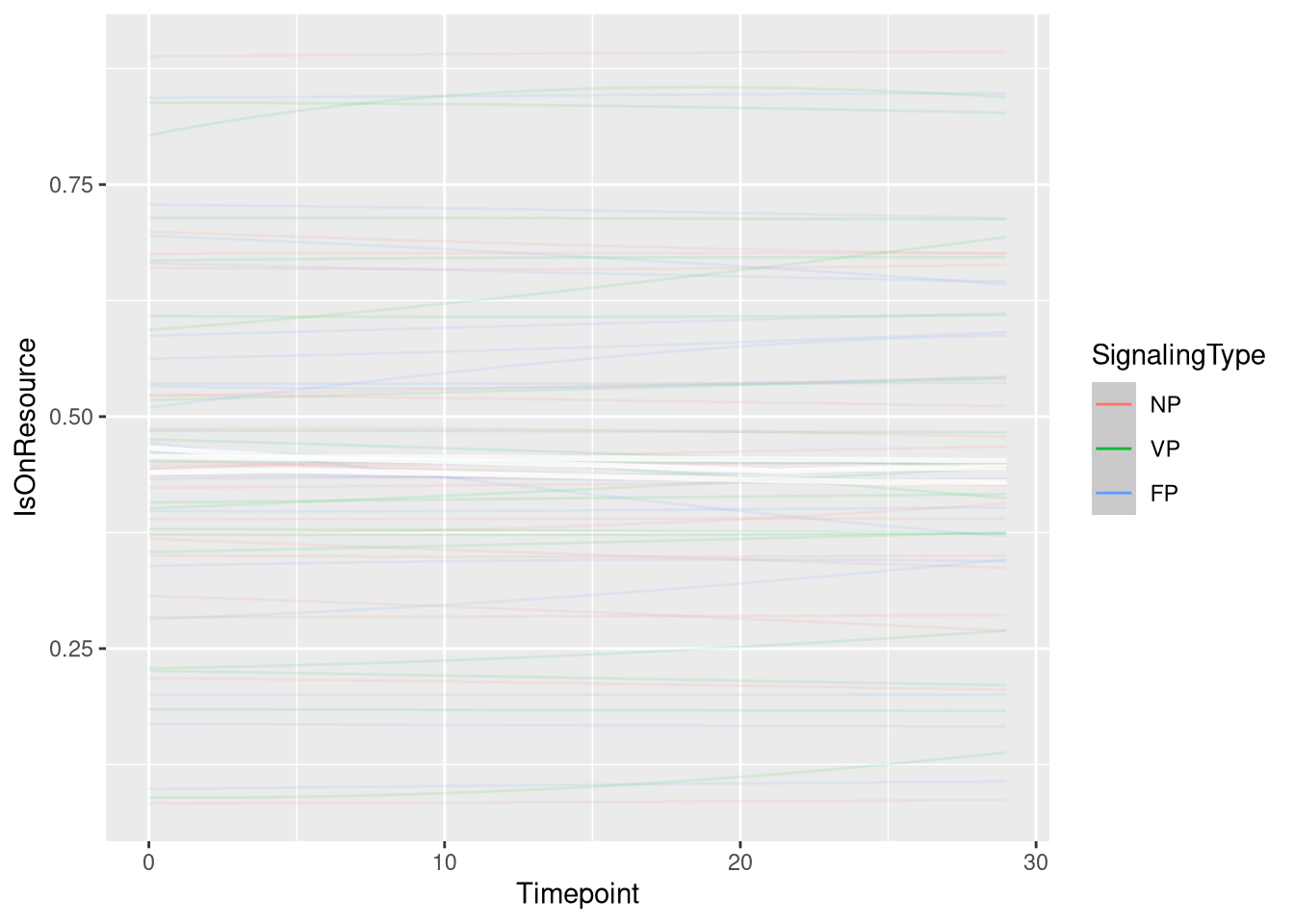
m.events.f.pstay.data <- resource_discoveries_data %>%
  filter(ResourceSpeed == 'fast', PlayerOrderCat == 'first') %>%
  filter(((Timepoint * 10) %% 10 == 0))
m.events.f.pstay.formula <- brmsformula(
IsOnResource ~ gp(Timepoint, by = SignalingType),
family = bernoulli(link = "logit")
)m.events.f.pstay.priors <-
prior(normal(0, 1), class = "Intercept") +
prior(inv_gamma(10, 20), class = "lscale", coef = "gpTimepointSignalingTypeA") +
prior(inv_gamma(10, 20), class = "lscale", coef = "gpTimepointSignalingTypeFP") +
prior(inv_gamma(10, 20), class = "lscale", coef = "gpTimepointSignalingTypeNP") +
prior(inv_gamma(10, 20), class = "lscale", coef = "gpTimepointSignalingTypeVP") +
prior(normal(0, 0.25), class = "sdgp", lb = 0)Prior predictive checks
m.events.f.pstay.fit_prior <- brm(
formula = m.events.f.pstay.formula,
prior = m.events.f.pstay.priors,
data = m.events.f.pstay.data,
seed = 42,
chains = 4,
cores = 4,
iter = 2000,
file = paste0(fits_path, 'resource_discoveries_fast_p_stay_prior.rds'),
backend = "cmdstanr",
threads = threading(100),
control = list(adapt_delta = 0.95),
save_pars = save_pars(all = TRUE),
sample_prior = "only"
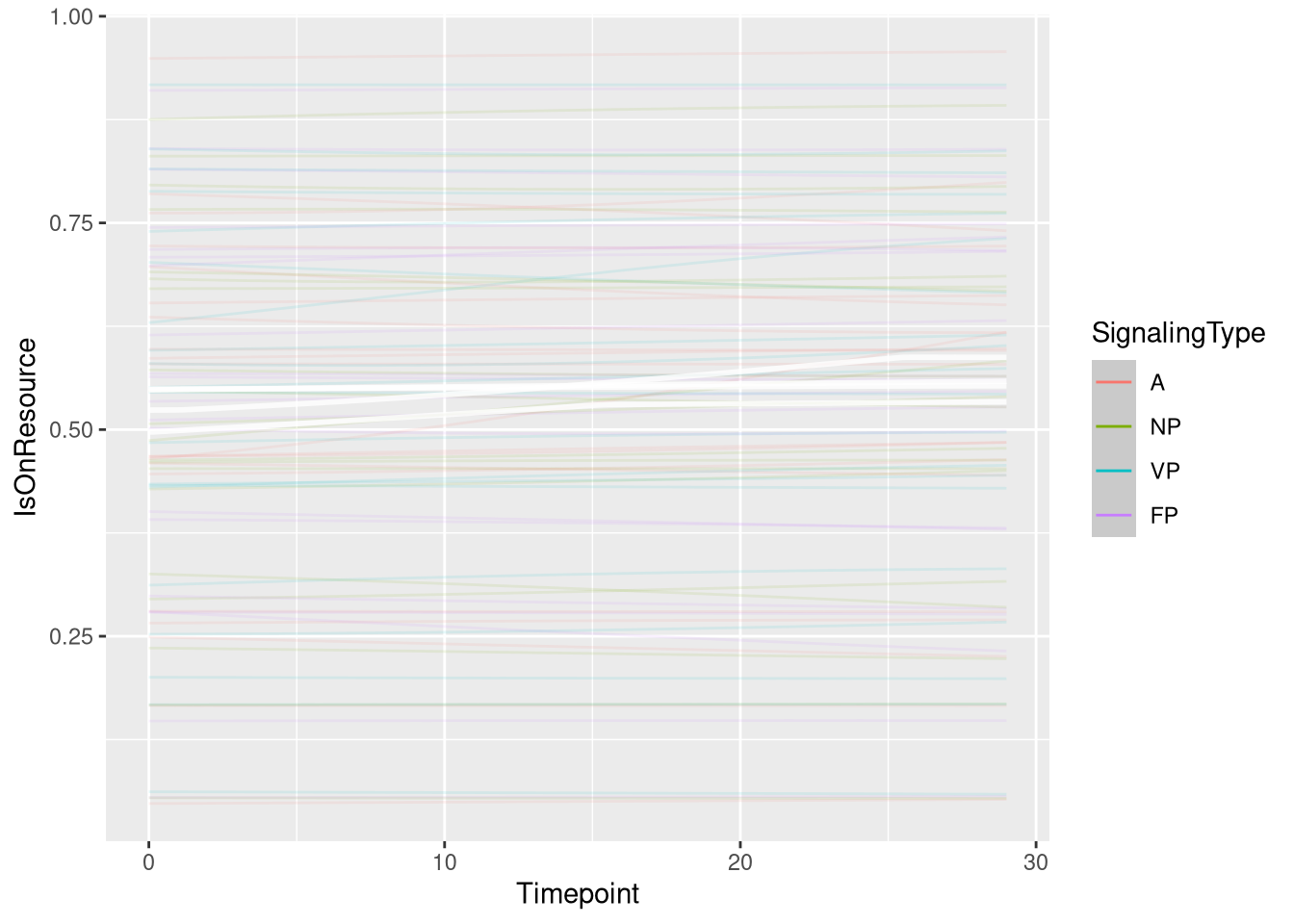
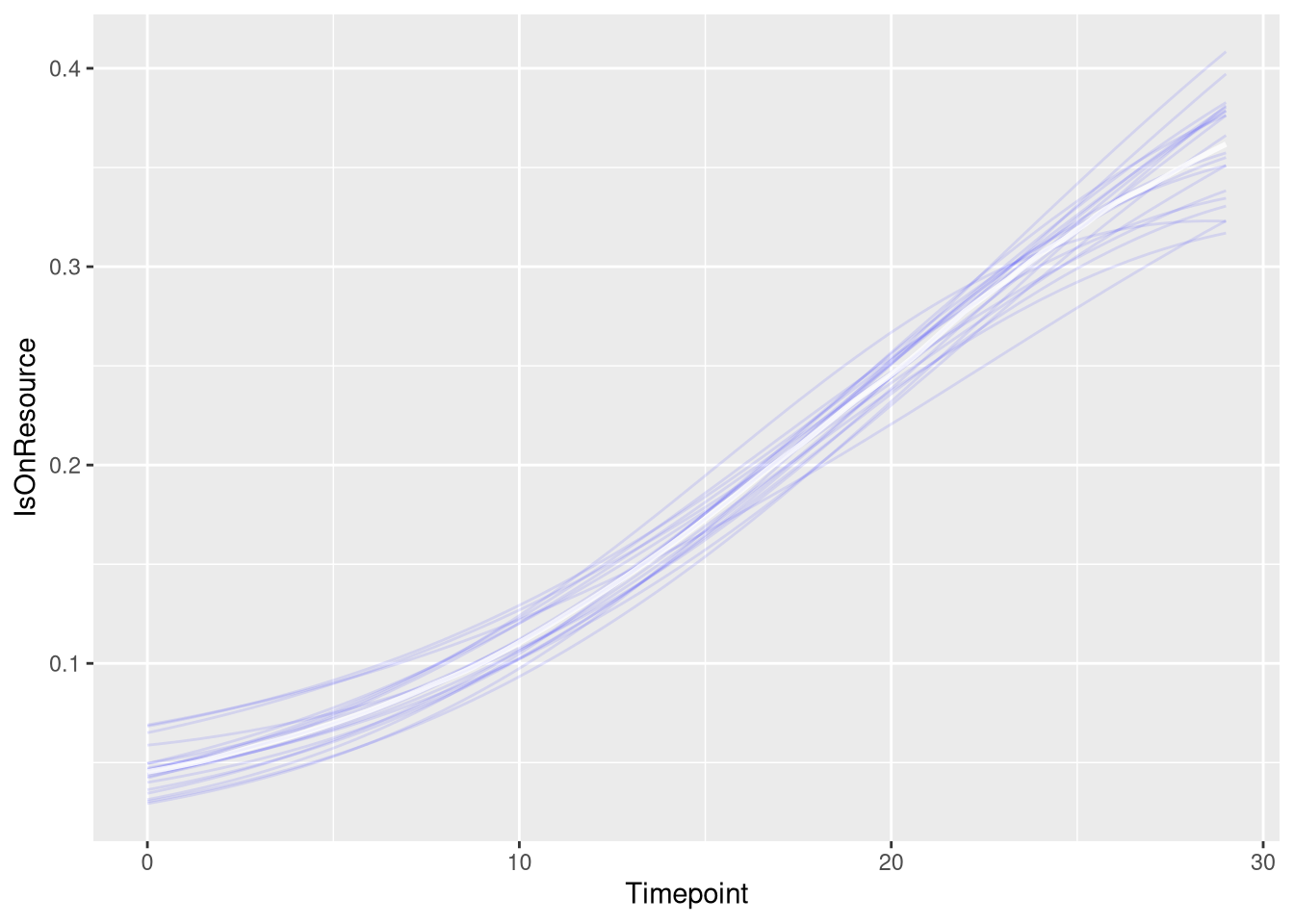
)plot(conditional_effects(m.events.f.pstay.fit_prior, ndraws = 20, spaghetti = TRUE), points = F, ask = F)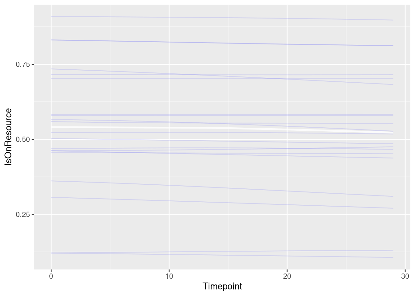
Model fitting
m.events.f.pstay.fit <- brm(
  formula = m.events.f.pstay.formula,
  prior   = m.events.f.pstay.priors,
  data    = m.events.f.pstay.data,
  chains = 4,
  cores = 4,
  seed = 42,
  warmup = 500,
  iter = 2000,
  file = paste0(fits_path, 'resource_discoveries_fast_p_stay.rds'),
  backend = "cmdstanr",
  threads = threading(100),
  control = list(adapt_delta = 0.95),
  save_pars = save_pars(all = TRUE)
)## Family: bernoulli
## Links: mu = logit
## Formula: IsOnResource ~ gp(Timepoint, by = SignalingType)
## Data: m.events.f.pstay.data (Number of observations: 24330)
## Draws: 4 chains, each with iter = 2000; warmup = 500; thin = 1;
## total post-warmup draws = 6000
##
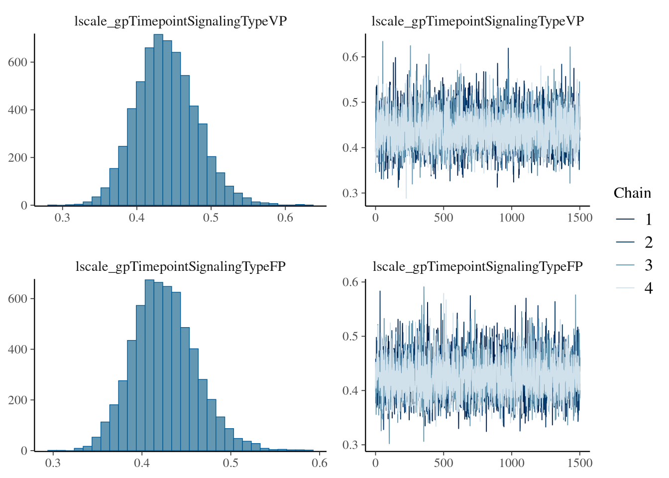
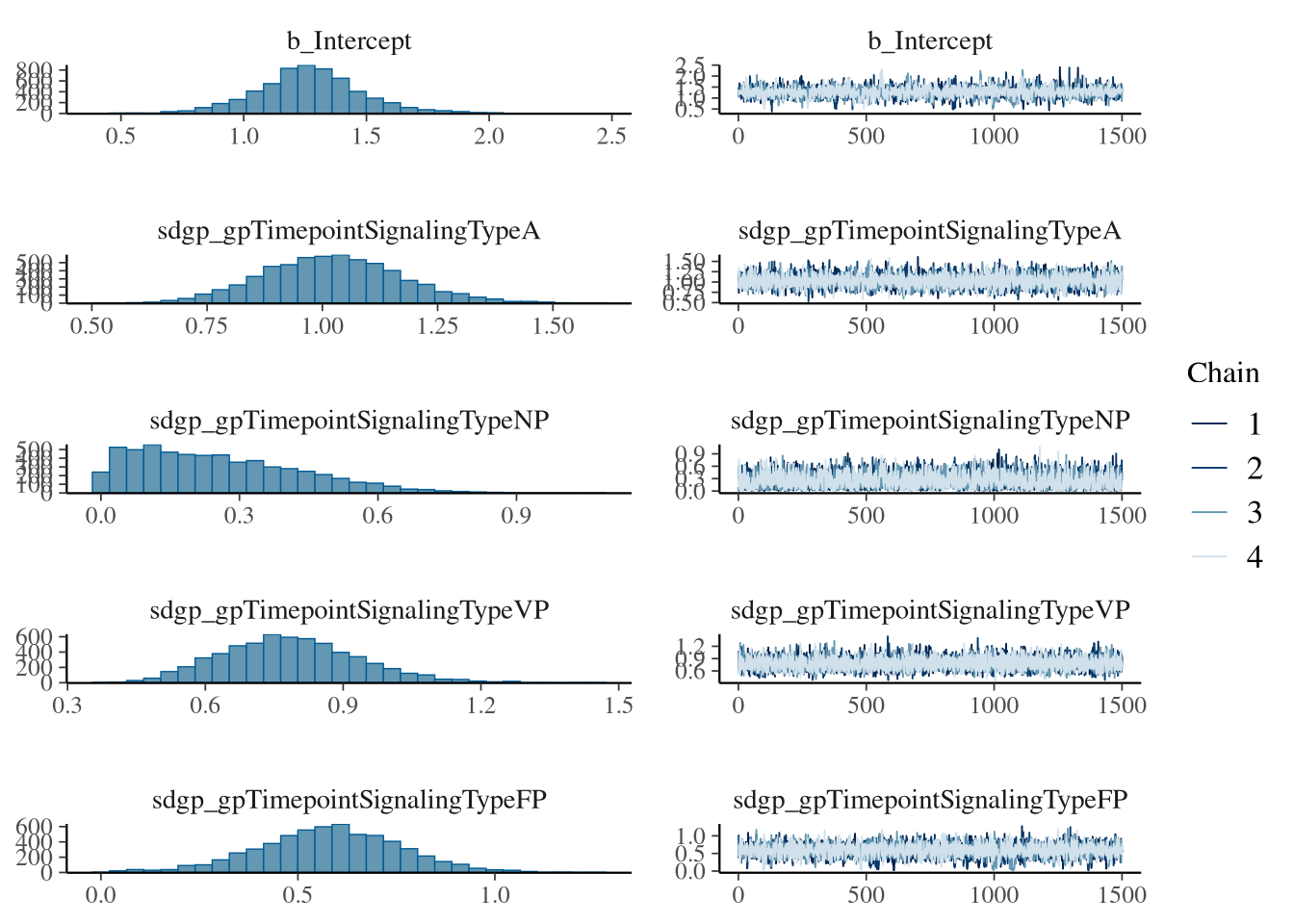
## Gaussian Process Hyperparameters:
## Estimate Est.Error l-95% CI u-95% CI Rhat Bulk_ESS Tail_ESS
## sdgp(gpTimepointSignalingTypeA) 1.25 0.15 0.98 1.56 1.00 6674 4196
## sdgp(gpTimepointSignalingTypeNP) 1.13 0.15 0.86 1.44 1.00 8307 3906
## sdgp(gpTimepointSignalingTypeVP) 1.17 0.15 0.89 1.47 1.00 8587 4806
## sdgp(gpTimepointSignalingTypeFP) 1.11 0.15 0.83 1.42 1.00 8121 4742
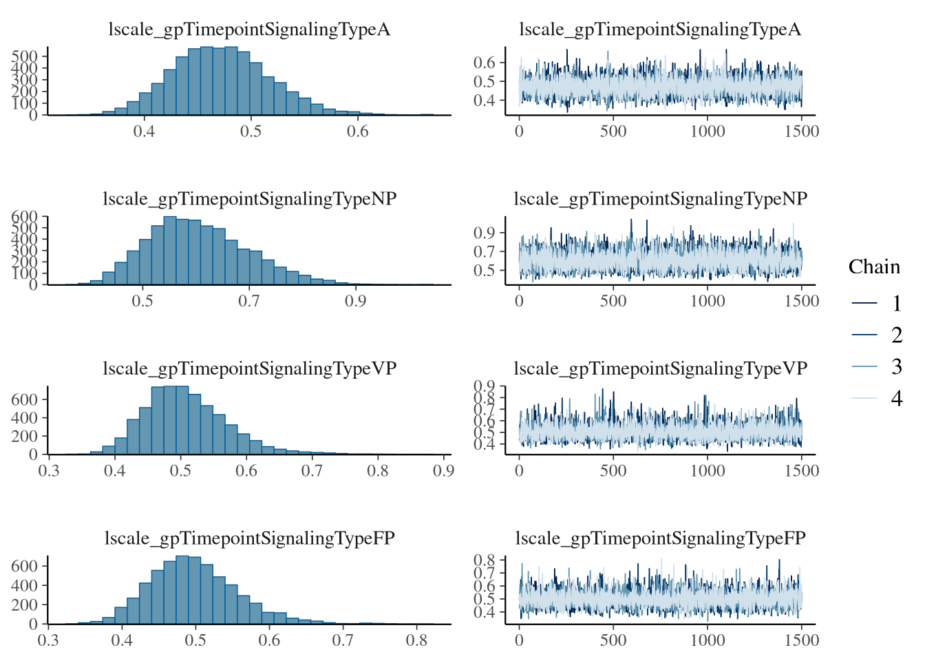
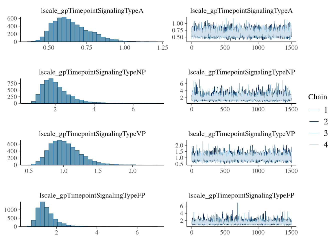
## lscale(gpTimepointSignalingTypeA) 0.47 0.05 0.39 0.57 1.00 6672 4882
## lscale(gpTimepointSignalingTypeNP) 0.61 0.09 0.45 0.81 1.00 4543 4725
## lscale(gpTimepointSignalingTypeVP) 0.51 0.06 0.40 0.65 1.00 5660 4320
## lscale(gpTimepointSignalingTypeFP) 0.50 0.06 0.40 0.63 1.00 6567 4588
##
## Regression Coefficients:
## Estimate Est.Error l-95% CI u-95% CI Rhat Bulk_ESS Tail_ESS
## Intercept 1.81 0.41 1.02 2.60 1.00 2757 3774
##
## Draws were sampled using sample(hmc). For each parameter, Bulk_ESS
## and Tail_ESS are effective sample size measures, and Rhat is the potential
## scale reduction factor on split chains (at convergence, Rhat = 1).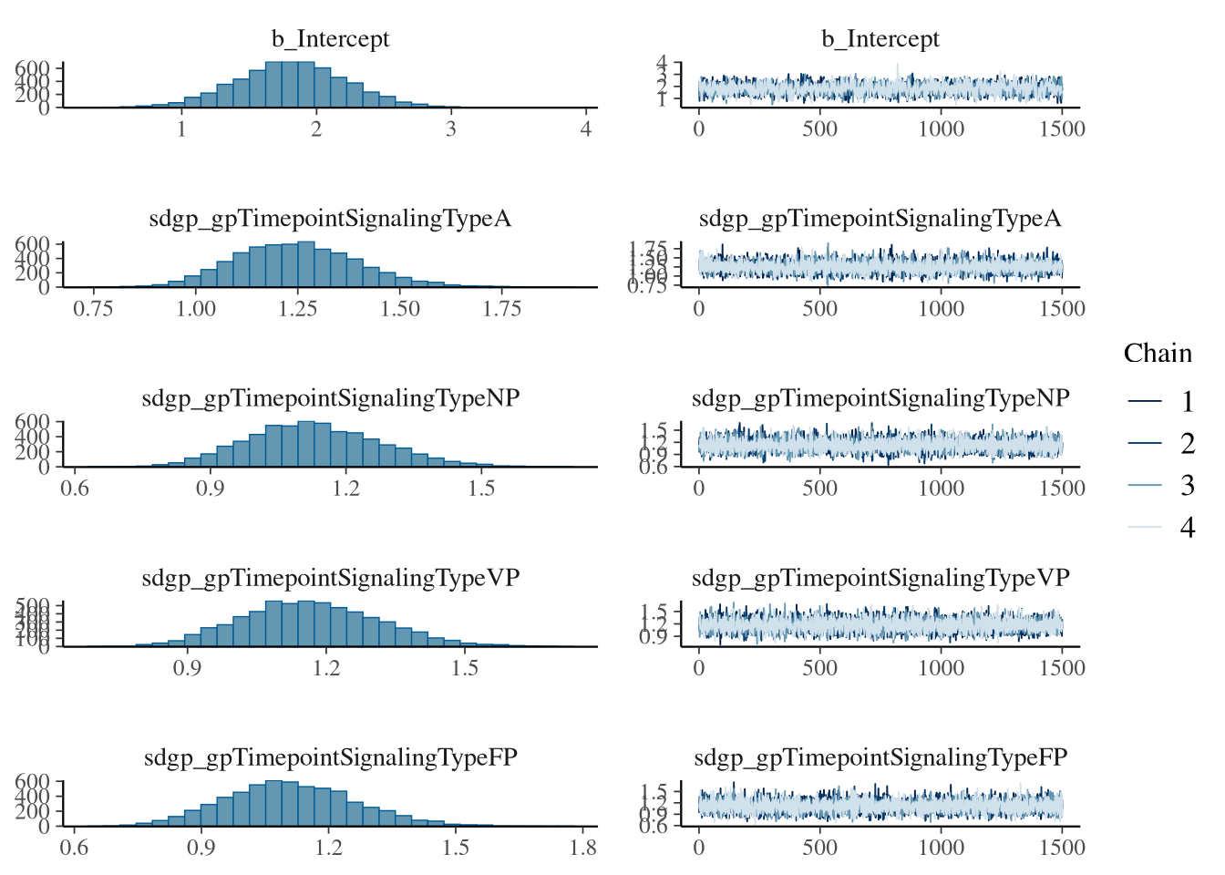
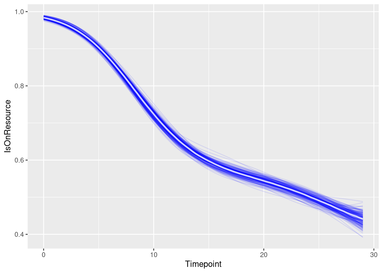
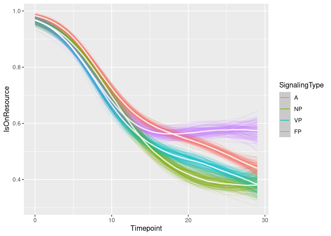
Figure
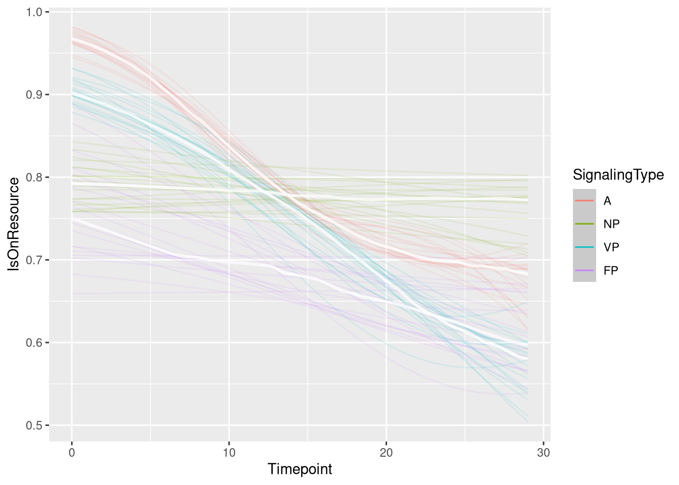
m.events.f.pstay.draws <- m.events.f.pstay.data %>%
mutate(SignalingType = factor(SignalingType, levels = c('A', 'NP', 'VP', 'FP'))) %>%
data_grid(Timepoint, SignalingType) %>%
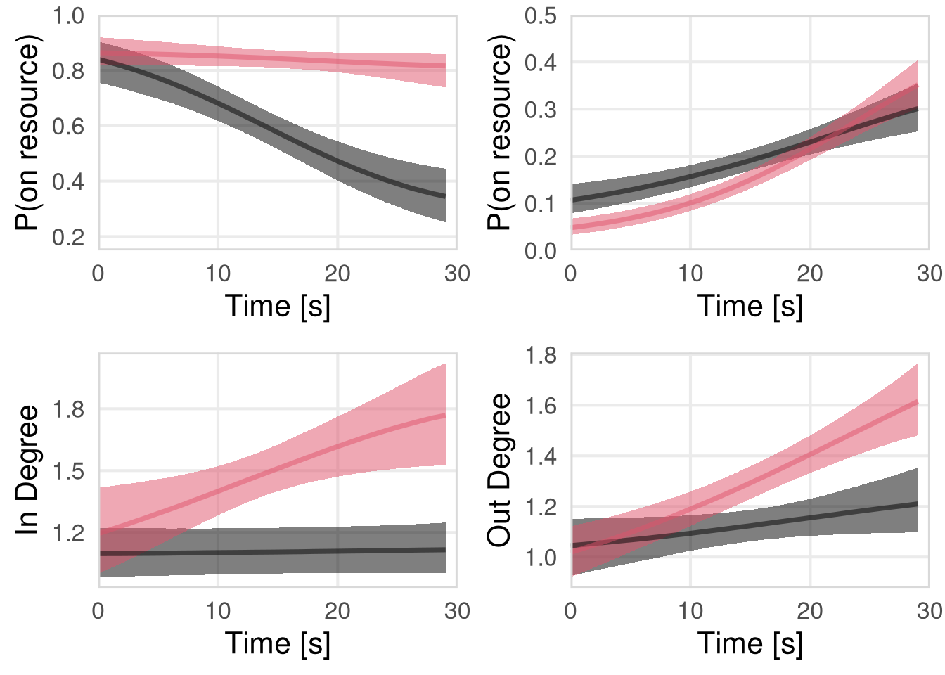
tidybayes::add_epred_draws(m.events.f.pstay.fit, allow_new_levels = TRUE, re_formula = m.events.f.pstay.formula)events_fast_p_stay_fig <- m.events.f.pstay.draws %>%
ggplot(aes(x = Timepoint, y = .epred, fill = SignalingType, color = SignalingType)) + # , group = SignalingType
stat_lineribbon(aes(group = paste(group, ...width..)), .width = c(.9), alpha = 1/2) +
# theme_nice(legend.pos = "top") +
theme_clean() +
panel_border() +
theme(legend.position = "none") +
scale_color_manual(breaks = c('A', 'NP', 'VP', 'FP'),
aesthetics = c("colour", "fill"),
values = c("#000000", "#DF536B", "#61D04F", "#2297E6"),
guide = guide_legend(
title = "Signaling",
)
) +
scale_y_continuous(
limits = c(0.25, 1.0),
expand = expansion(mult = c(0, 0))
) +
scale_x_continuous(
limits = c(0, 30),
expand = expansion(mult = c(0, 0))
) +
labs(x = "Time [s]",
y = "P(on resource)") # Probability of being on resource (first player)
events_fast_p_stay_fig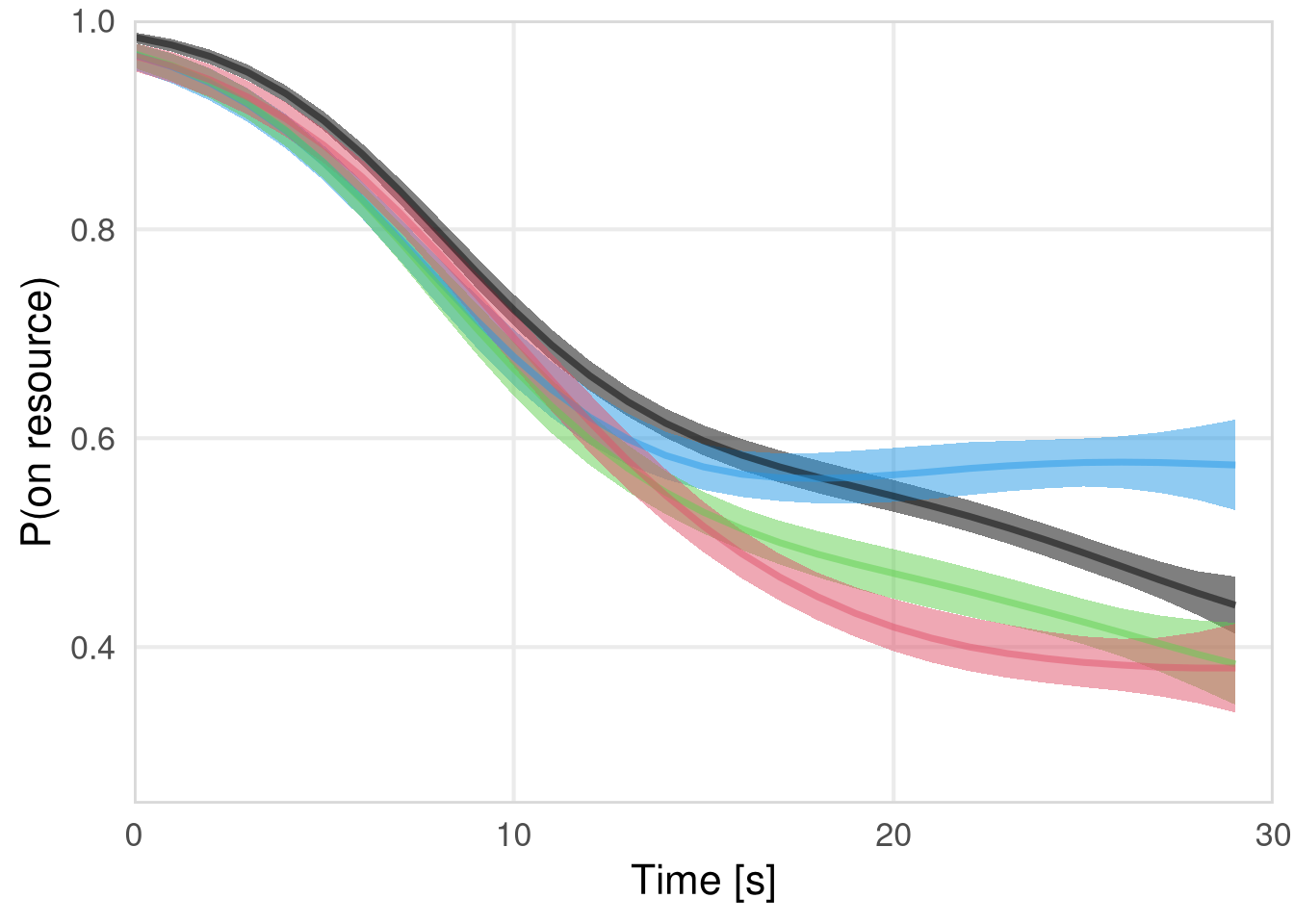
Probability of staying on resource VP
m.events.f.pstay.VP.data <- resource_discoveries_data_vp %>%
  filter(ResourceSpeed == 'fast', PlayerOrderCat == 'first') %>%
  filter(((Timepoint * 10) %% 10 == 0))
m.events.f.pstay.VP.formula <- brmsformula(
IsOnResource ~ gp(Timepoint, by = SignalingType),
family = bernoulli(link = "logit")
)m.events.f.pstay.VP.priors <-
prior(normal(0, 1), class = "Intercept") +
prior(inv_gamma(10, 20), class = "lscale", coef = "gpTimepointSignalingTypeVP_NS") +
prior(inv_gamma(10, 20), class = "lscale", coef = "gpTimepointSignalingTypeVP_S") +
prior(normal(0, 0.25), class = "sdgp", lb = 0)Prior predictive checks
m.events.f.pstay.VP.fit_prior <- brm(
  formula = m.events.f.pstay.VP.formula,
  prior   = m.events.f.pstay.VP.priors,
  data    = m.events.f.pstay.VP.data,
  seed    = 42,
  chains  = 4,
  cores   = 4,
  iter    = 2000,
  file = paste0(fits_path, 'resource_discoveries_fast_p_stay_vp_prior.rds'),
  backend = "cmdstanr",
  threads = threading(100),
  control = list(adapt_delta = 0.95),
  save_pars = save_pars(all = TRUE),
  sample_prior = "only"
)plot(conditional_effects(m.events.f.pstay.VP.fit_prior, ndraws = 20, spaghetti = TRUE), points = F, ask = F)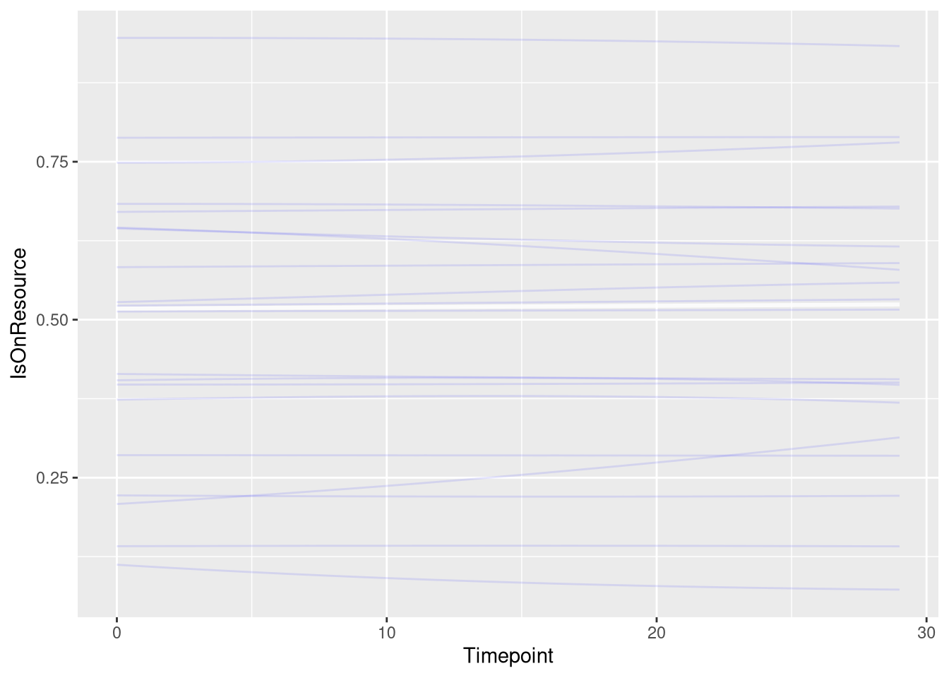
Model fitting
m.events.f.pstay.VP.fit <- brm(
  formula = m.events.f.pstay.VP.formula,
  prior   = m.events.f.pstay.VP.priors,
  data    = m.events.f.pstay.VP.data,
  chains = 4,
  cores = 4,
  seed = 42,
  warmup = 500,
  iter = 2000,
  file = paste0(fits_path, 'resource_discoveries_fast_p_stay_vp.rds'),
  backend = "cmdstanr",
  threads = threading(100),
  control = list(adapt_delta = 0.95),
  save_pars = save_pars(all = TRUE)
)## Family: bernoulli
## Links: mu = logit
## Formula: IsOnResource ~ gp(Timepoint, by = SignalingType)
## Data: m.events.f.pstay.VP.data (Number of observations: 5010)
## Draws: 4 chains, each with iter = 2000; warmup = 500; thin = 1;
## total post-warmup draws = 6000
##
## Gaussian Process Hyperparameters:
## Estimate Est.Error l-95% CI u-95% CI Rhat Bulk_ESS Tail_ESS
## sdgp(gpTimepointSignalingTypeVP_NS) 1.12 0.15 0.85 1.43 1.00 10306 4790
## sdgp(gpTimepointSignalingTypeVP_S) 0.92 0.14 0.66 1.22 1.00 10716 4607
## lscale(gpTimepointSignalingTypeVP_NS) 0.60 0.09 0.45 0.79 1.00 5414 4021
## lscale(gpTimepointSignalingTypeVP_S) 0.92 0.15 0.67 1.25 1.00 8449 4345
##
## Regression Coefficients:
## Estimate Est.Error l-95% CI u-95% CI Rhat Bulk_ESS Tail_ESS
## Intercept 1.40 0.51 0.40 2.45 1.00 5179 3906
##
## Draws were sampled using sample(hmc). For each parameter, Bulk_ESS
## and Tail_ESS are effective sample size measures, and Rhat is the potential
## scale reduction factor on split chains (at convergence, Rhat = 1).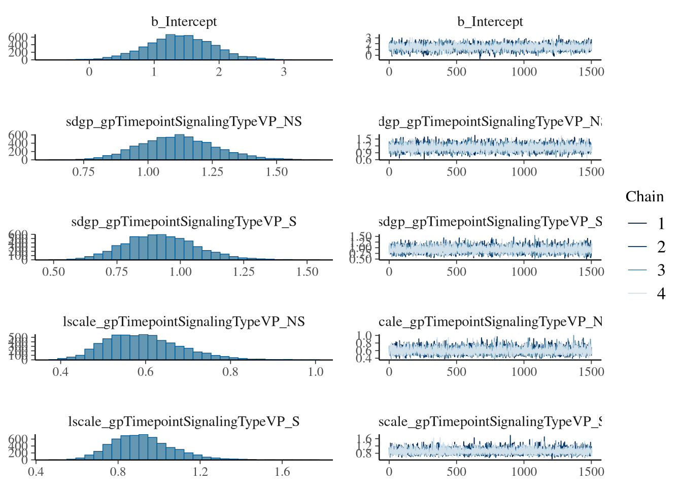
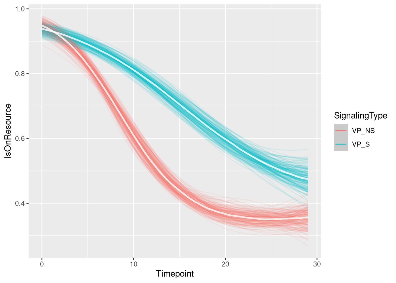
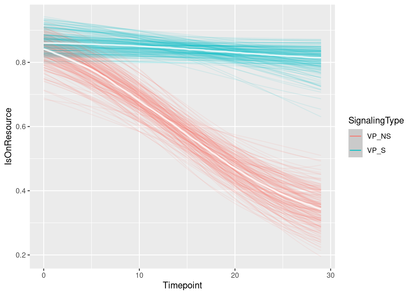
Figure
m.events.f.pstay.VP.draws <- m.events.f.pstay.VP.data %>%
  mutate(SignalingType = factor(SignalingType, levels = c('VP_NS', 'VP_S'))) %>%
  data_grid(Timepoint, SignalingType) %>%
  tidybayes::add_epred_draws(m.events.f.pstay.VP.fit, allow_new_levels = TRUE, re_formula = m.events.f.pstay.VP.formula)
events_fast_p_stay_vp_fig <- m.events.f.pstay.VP.draws %>%
ggplot(aes(x = Timepoint, y = .epred, fill = SignalingType, color = SignalingType)) + # , group = SignalingType
stat_lineribbon(aes(group = paste(group, ...width..)), .width = c(.9), alpha = 1/2) +
theme_clean() +
panel_border() +
theme(legend.position = "none") +
scale_color_manual(breaks = c('VP_NS', 'VP_S'),
aesthetics = c("colour", "fill"),
values = c("#000000", "#DF536B"),
guide = guide_legend(
title = "Signaling",
)
) +
scale_y_continuous(
limits = c(0.25, 1.0),
expand = expansion(mult = c(0, 0))
) +
scale_x_continuous(
limits = c(0, 30),
expand = expansion(mult = c(0, 0))
) +
labs(x = "Time [s]",
y = "P(on resource)")
events_fast_p_stay_vp_fig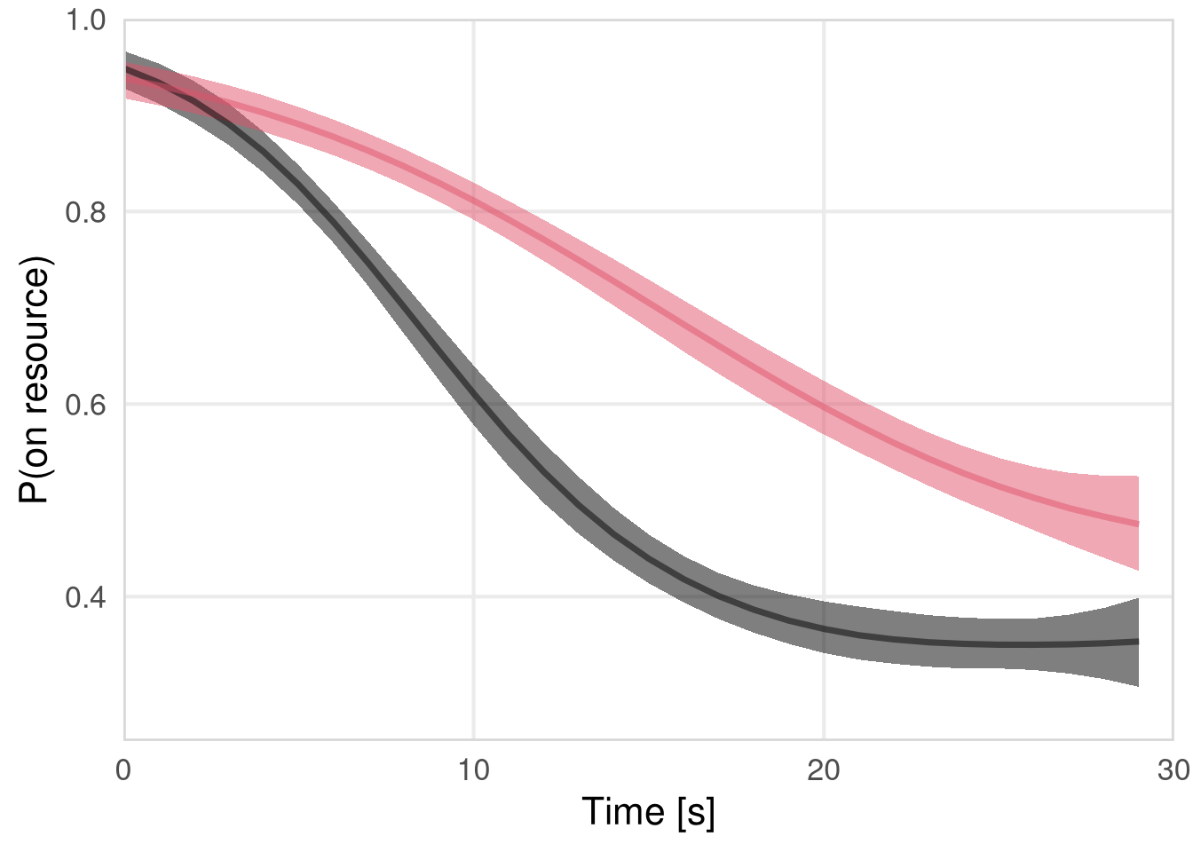
Probability of reaching resource
m.events.f.reach.data <- resource_discoveries_data %>%
  filter(ResourceSpeed == 'fast', SignalingType != 'A', PlayerOrderCat == 'others') %>%
  filter(((Timepoint * 10) %% 10 == 0))


m.events.f.reach.formula <- brmsformula(
  IsOnResource ~ gp(Timepoint, by = SignalingType),
  family = bernoulli(link = "logit")
  )
m.events.f.reach.priors <-
prior(normal(0, 1), class = "Intercept") +
prior(inv_gamma(10, 20), class = "lscale", coef = "gpTimepointSignalingTypeFP") +
prior(inv_gamma(10, 20), class = "lscale", coef = "gpTimepointSignalingTypeNP") +
prior(inv_gamma(10, 20), class = "lscale", coef = "gpTimepointSignalingTypeVP") +
prior(normal(0, 0.25), class = "sdgp", lb = 0)Prior predictive checks
m.events.f.reach.fit_prior <- brm(
  formula = m.events.f.reach.formula,
  prior   = m.events.f.reach.priors,
  data    = m.events.f.reach.data,
  chains  = 4,
  cores   = 4,
  seed    = 42,
  iter    = 2000,
  file = paste0(fits_path, 'resource_discoveries_fast_p_reach_prior.rds'),
  backend = "cmdstanr",
  threads = threading(100),
  control = list(adapt_delta = 0.95),
  save_pars = save_pars(all = TRUE),
  sample_prior = "only"
)plot(conditional_effects(m.events.f.reach.fit_prior, ndraws = 20, spaghetti = TRUE), points = F, ask = F)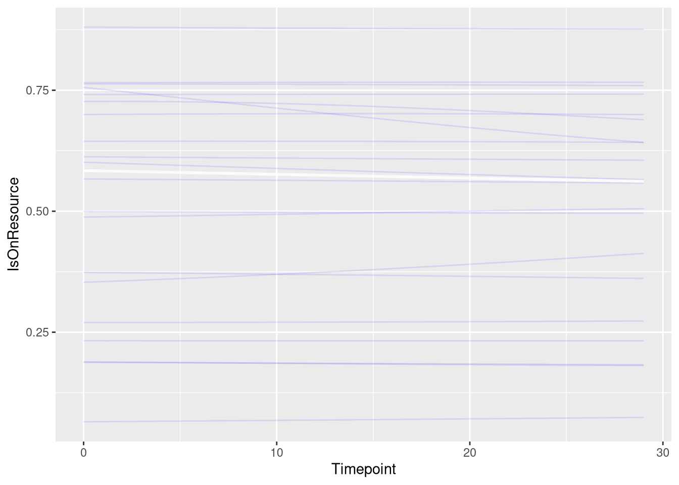
Model fitting
m.events.f.reach.fit <- brm(
  formula = m.events.f.reach.formula,
  prior   = m.events.f.reach.priors,
  data    = m.events.f.reach.data,
  chains = 4,
  cores = 4,
  seed = 42,
  warmup = 500,
  iter = 2000,
  file = paste0(fits_path, 'resource_discoveries_fast_p_reach.rds'),
  backend = "cmdstanr",
  threads = threading(100),
  control = list(adapt_delta = 0.95),
  save_pars = save_pars(all = TRUE)
)## Family: bernoulli
## Links: mu = logit
## Formula: IsOnResource ~ gp(Timepoint, by = SignalingType)
## Data: m.events.f.reach.data (Number of observations: 47910)
## Draws: 4 chains, each with iter = 2000; warmup = 500; thin = 1;
## total post-warmup draws = 6000
##
## Gaussian Process Hyperparameters:
## Estimate Est.Error l-95% CI u-95% CI Rhat Bulk_ESS Tail_ESS
## sdgp(gpTimepointSignalingTypeNP) 0.99 0.15 0.72 1.32 1.00 5555 4240
## sdgp(gpTimepointSignalingTypeVP) 1.11 0.15 0.83 1.43 1.00 4518 4285
## sdgp(gpTimepointSignalingTypeFP) 1.17 0.15 0.89 1.48 1.00 5339 4509
## lscale(gpTimepointSignalingTypeNP) 0.62 0.09 0.46 0.83 1.00 6123 4681
## lscale(gpTimepointSignalingTypeVP) 0.44 0.04 0.37 0.53 1.00 5420 4760
## lscale(gpTimepointSignalingTypeFP) 0.43 0.04 0.36 0.50 1.00 4666 4500
##
## Regression Coefficients:
## Estimate Est.Error l-95% CI u-95% CI Rhat Bulk_ESS Tail_ESS
## Intercept -2.34 0.40 -3.14 -1.53 1.00 2027 3164
##
## Draws were sampled using sample(hmc). For each parameter, Bulk_ESS
## and Tail_ESS are effective sample size measures, and Rhat is the potential
## scale reduction factor on split chains (at convergence, Rhat = 1).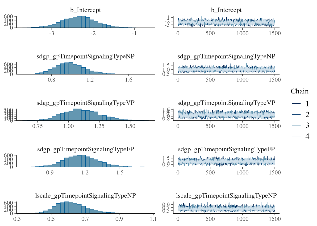
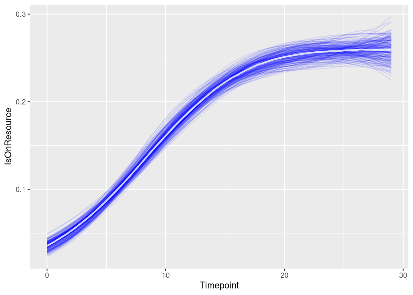
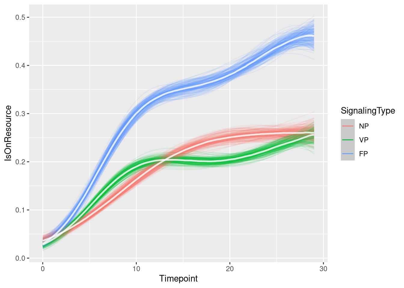
Figure
m.events.f.reach.draws <- m.events.f.reach.data %>%
  mutate(SignalingType = factor(SignalingType, levels = c('NP', 'VP', 'FP'))) %>%
  data_grid(Timepoint, SignalingType) %>%
  tidybayes::add_epred_draws(m.events.f.reach.fit, allow_new_levels = TRUE, re_formula = m.events.f.reach.formula)
events_fast_p_reach_fig <- m.events.f.reach.draws %>%
ggplot(aes(x = Timepoint, y = .epred, fill = SignalingType, color = SignalingType)) + # , group = SignalingType
stat_lineribbon(aes(group = paste(group, ...width..)), .width = c(.9), alpha = 1/2) +
scale_color_manual(breaks = c('NP', 'VP', 'FP'),
aesthetics = c("colour", "fill"),
values = c("#DF536B", "#61D04F", "#2297E6"),
guide = guide_legend(
title = "Signaling",
)
) +
# theme_nice(legend.pos = 'top') +
theme_clean() +
panel_border() +
theme(legend.position = "none") +
scale_y_continuous(
limits = c(0, 0.5),
expand = expansion(mult = c(0, 0))
) +
scale_x_continuous(
limits = c(0, 30),
expand = expansion(mult = c(0, 0))
) +
labs(x = "Time [s]",
y = "P(on resource)") # "Probability of being on resource (other players)"
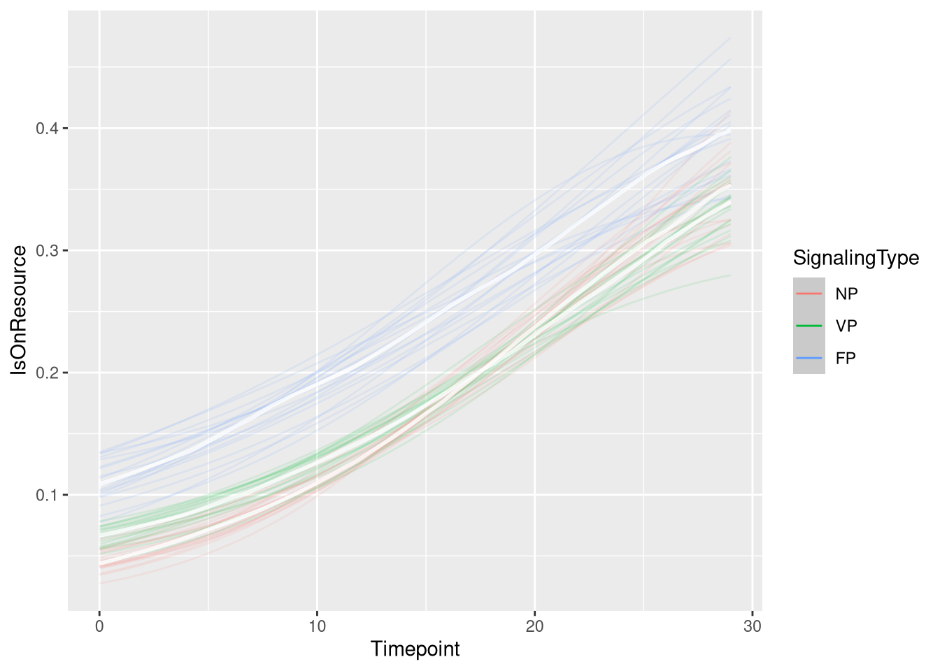
events_fast_p_reach_fig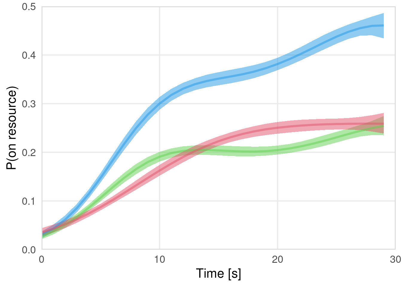
Probability of reaching resource VP
m.events.f.reach.VP.data <- resource_discoveries_data_vp %>%
  filter(ResourceSpeed == 'fast', PlayerOrderCat == 'others') %>%
  filter(((Timepoint * 10) %% 10 == 0))


m.events.f.reach.VP.formula <- brmsformula(
  IsOnResource ~ gp(Timepoint, by = SignalingType),
  family = bernoulli(link = "logit")
  )
m.events.f.reach.VP.priors <-
prior(normal(0, 1), class = "Intercept") +
prior(inv_gamma(10, 20), class = "lscale", coef = "gpTimepointSignalingTypeVP_NS") +
prior(inv_gamma(10, 20), class = "lscale", coef = "gpTimepointSignalingTypeVP_S") +
prior(normal(0, 0.25), class = "sdgp", lb = 0)Prior predictive checks
m.events.f.reach.VP.fit_prior <- brm(
  formula = m.events.f.reach.VP.formula,
  prior   = m.events.f.reach.VP.priors,
  data    = m.events.f.reach.VP.data,
  chains  = 4,
  cores   = 4,
  seed    = 42,
  iter    = 2000,
  file = paste0(fits_path, 'resource_discoveries_fast_p_reach_vp_prior.rds'),
  backend = "cmdstanr",
  threads = threading(100),
  control = list(adapt_delta = 0.95),
  save_pars = save_pars(all = TRUE),
  sample_prior = "only"
)plot(conditional_effects(m.events.f.reach.VP.fit_prior, ndraws = 20, spaghetti = TRUE), points = F, ask = F)
Model fitting
m.events.f.reach.VP.fit <- brm(
  formula = m.events.f.reach.VP.formula,
  prior   = m.events.f.reach.VP.priors,
  data    = m.events.f.reach.VP.data,
  chains = 4,
  cores = 4,
  seed = 42,
  warmup = 500,
  iter = 2000,
  file = paste0(fits_path, 'resource_discoveries_fast_p_reach_vp.rds'),
  backend = "cmdstanr",
  threads = threading(100),
  control = list(adapt_delta = 0.95),
  save_pars = save_pars(all = TRUE)
)## Family: bernoulli
## Links: mu = logit
## Formula: IsOnResource ~ gp(Timepoint, by = SignalingType)
## Data: m.events.f.reach.VP.data (Number of observations: 18480)
## Draws: 4 chains, each with iter = 2000; warmup = 500; thin = 1;
## total post-warmup draws = 6000
##
## Gaussian Process Hyperparameters:
## Estimate Est.Error l-95% CI u-95% CI Rhat Bulk_ESS Tail_ESS
## sdgp(gpTimepointSignalingTypeVP_NS) 1.03 0.16 0.75 1.35 1.00 5009 4151
## sdgp(gpTimepointSignalingTypeVP_S) 0.91 0.15 0.64 1.24 1.00 5088 3649
## lscale(gpTimepointSignalingTypeVP_NS) 0.48 0.05 0.39 0.57 1.00 5395 4640
## lscale(gpTimepointSignalingTypeVP_S) 0.77 0.15 0.50 1.07 1.00 3454 4529
##
## Regression Coefficients:
## Estimate Est.Error l-95% CI u-95% CI Rhat Bulk_ESS Tail_ESS
## Intercept -2.04 0.48 -2.94 -1.09 1.00 2377 3455
##
## Draws were sampled using sample(hmc). For each parameter, Bulk_ESS
## and Tail_ESS are effective sample size measures, and Rhat is the potential
## scale reduction factor on split chains (at convergence, Rhat = 1).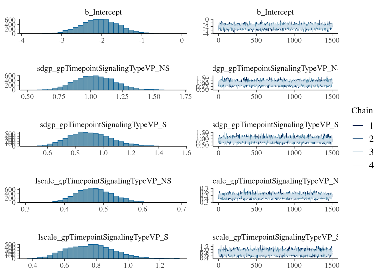
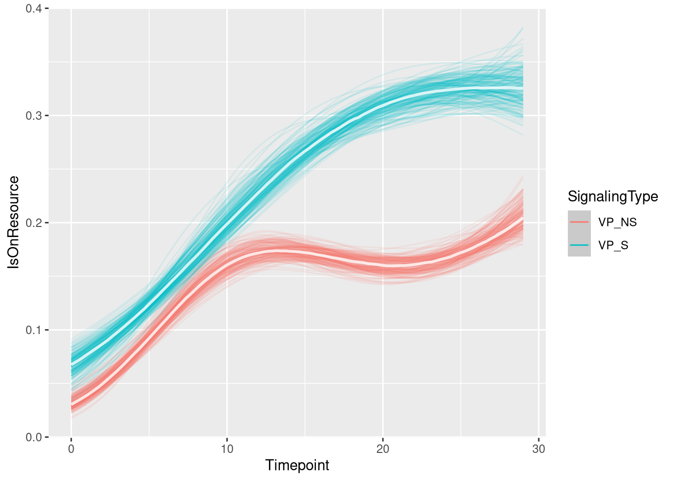
Figure
m.events.f.reach.VP.draws <- m.events.f.reach.VP.data %>%
  mutate(SignalingType = factor(SignalingType, levels = c('VP_NS', 'VP_S'))) %>%
  data_grid(Timepoint, SignalingType) %>%
  tidybayes::add_epred_draws(m.events.f.reach.VP.fit, allow_new_levels = TRUE, re_formula = m.events.f.reach.VP.formula)
events_fast_p_reach_vp_fig <- m.events.f.reach.VP.draws %>%
ggplot(aes(x = Timepoint, y = .epred, fill = SignalingType, color = SignalingType)) + # , group = SignalingType
stat_lineribbon(aes(group = paste(group, ...width..)), .width = c(.9), alpha = 1/2) +
theme_nice(legend.pos = 'top') +
scale_color_manual(breaks = c('VP_NS', 'VP_S'),
aesthetics = c("colour", "fill"),
values = c("#000000", "#DF536B"),
guide = guide_legend(
title = "Signaling",
)
) +
theme_clean() +
panel_border() +
theme(legend.position = "none") +
scale_y_continuous(
limits = c(0, 0.4),
expand = expansion(mult = c(0, 0))
) +
scale_x_continuous(
limits = c(0, 30),
expand = expansion(mult = c(0, 0))
) +
labs(x = "Time [s]",
y = "P(on resource)")
events_fast_p_reach_vp_fig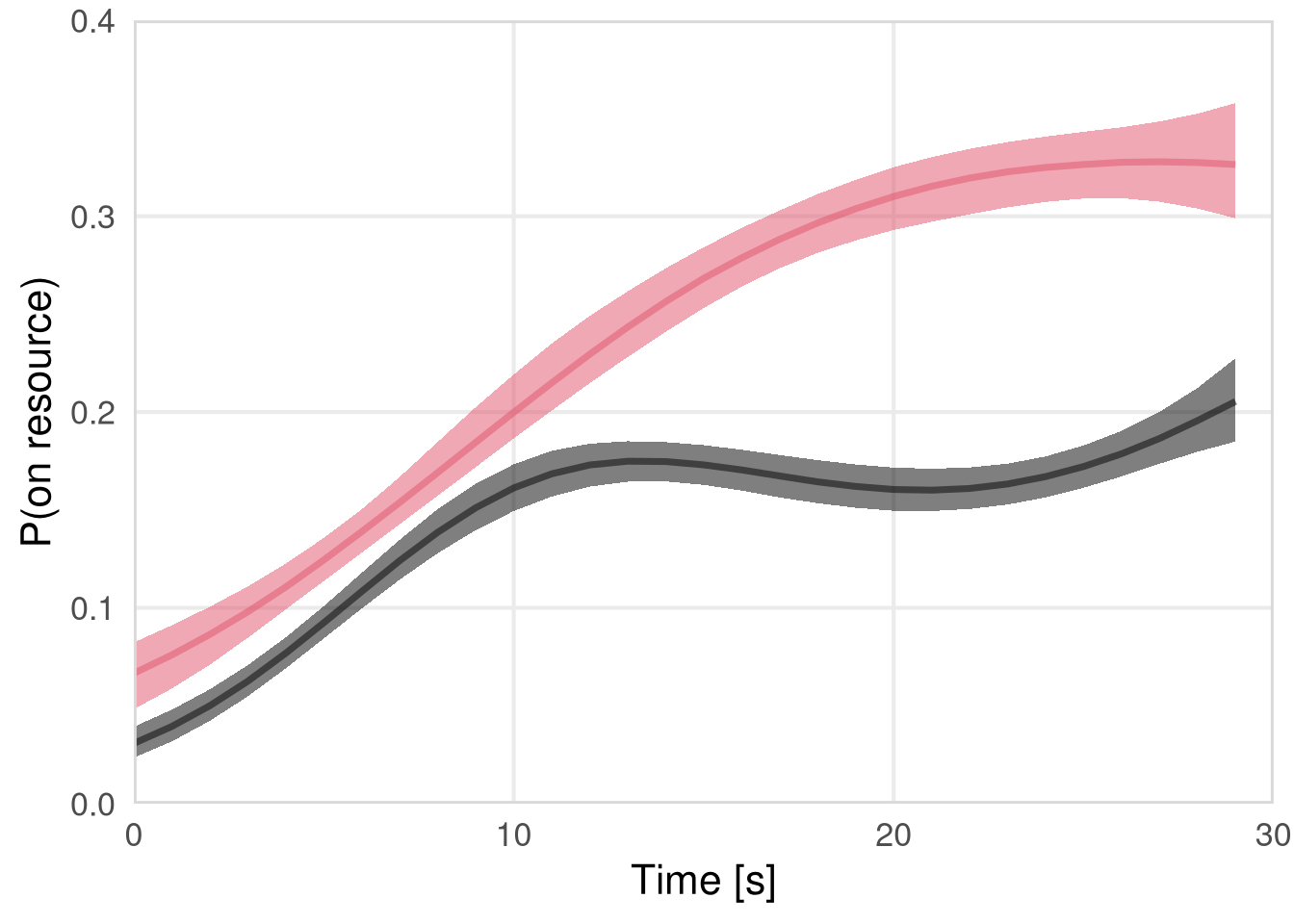
Out degree
m.events.f.OutDegree.data  <- resource_discoveries_data %>%
  filter(ResourceSpeed == 'fast', SignalingType != 'A', PlayerOrderCat == 'others') %>%
  filter(((Timepoint * 10) %% 10 == 0))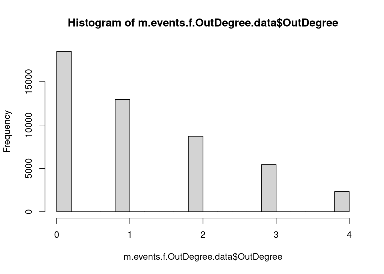
m.events.f.OutDegree.formula <- brmsformula(
  OutDegree ~ gp(Timepoint, by = SignalingType),
  family = poisson(link = "log")
  )
m.events.f.OutDegree.priors <-
prior(normal(0, 1), class = "Intercept") +
prior(inv_gamma(10, 20), class = "lscale", coef = "gpTimepointSignalingTypeFP") +
prior(inv_gamma(10, 20), class = "lscale", coef = "gpTimepointSignalingTypeNP") +
prior(inv_gamma(10, 20), class = "lscale", coef = "gpTimepointSignalingTypeVP") +
prior(normal(0, 0.25), class = "sdgp", lb = 0)Prior predictive checks
m.events.f.OutDegree.fit_prior <- brm(
  formula = m.events.f.OutDegree.formula,
  family = poisson(link = "log"),
  prior = m.events.f.OutDegree.priors,
  m.events.f.OutDegree.data,
  chains  = 4,
  cores   = 4,
  seed    = 42,
  iter    = 2000,
  file = paste0(fits_path, 'resource_discoveries_fast_out_degree._prior.rds'),
  backend = "cmdstanr",
  threads = threading(100),
  control = list(adapt_delta = 0.95),
  save_pars = save_pars(all = TRUE),
  sample_prior = "only"
)plot(conditional_effects(m.events.f.OutDegree.fit_prior, ndraws = 20, spaghetti = TRUE), points = F, ask = F)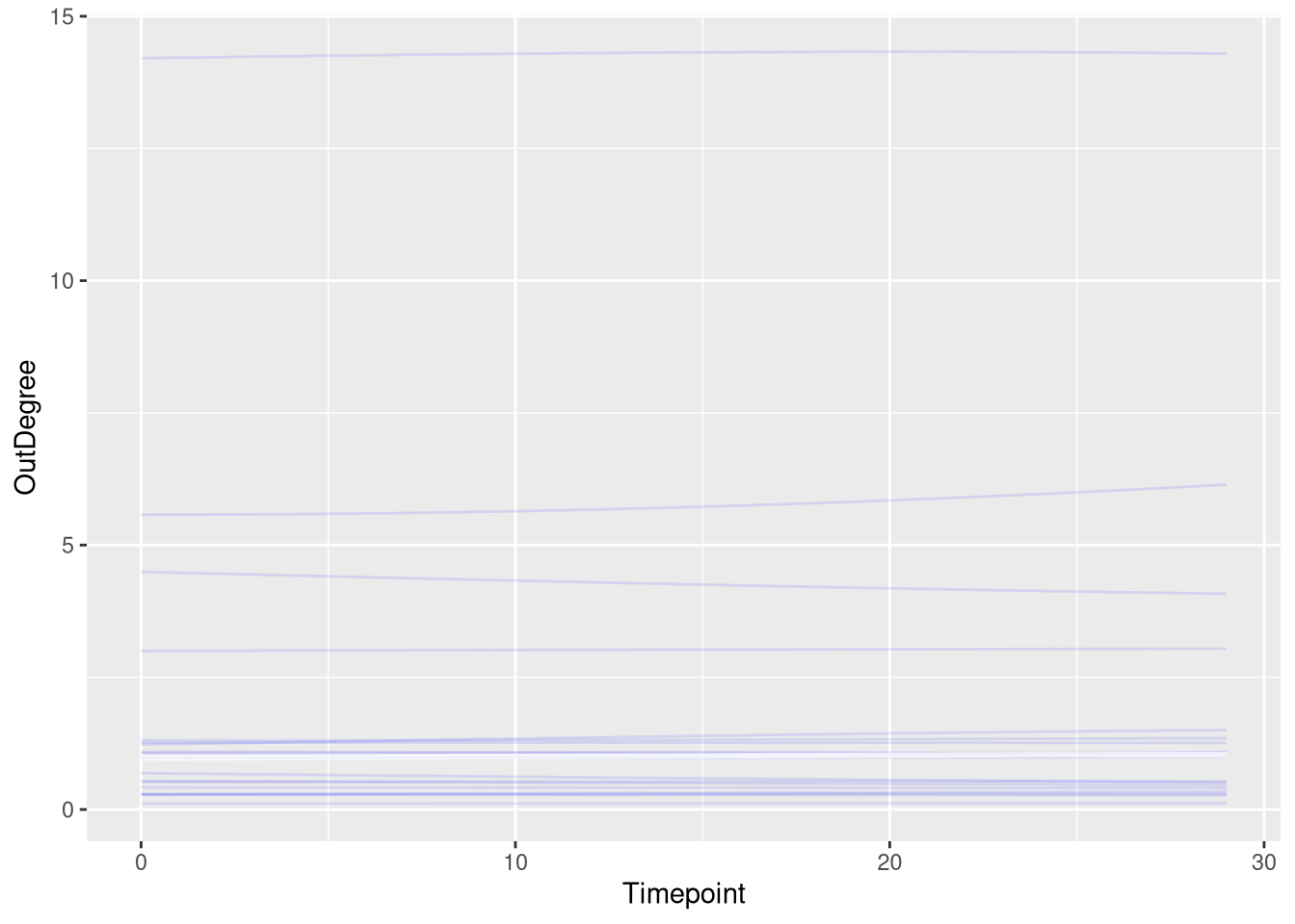
Model fitting
m.events.f.OutDegree.fit <- brm(
  formula = m.events.f.OutDegree.formula,
  prior   = m.events.f.OutDegree.priors,
  data    = m.events.f.OutDegree.data ,
  chains = 4,
  cores = 4,
  seed = 42,
  warmup = 500,
  iter = 2000,
  file = paste0(fits_path, 'resource_discoveries_fast_out_degree.rds'),
  backend = "cmdstanr",
  threads = threading(100),
  control = list(adapt_delta = 0.95),
  save_pars = save_pars(all = TRUE)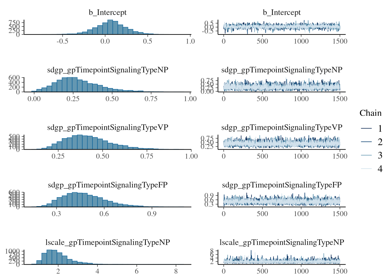
)## Family: poisson
## Links: mu = log
## Formula: OutDegree ~ gp(Timepoint, by = SignalingType)
## Data: m.events.f.OutDegree.data (Number of observations: 47910)
## Draws: 4 chains, each with iter = 2000; warmup = 500; thin = 1;
## total post-warmup draws = 6000
##
## Gaussian Process Hyperparameters:
## Estimate Est.Error l-95% CI u-95% CI Rhat Bulk_ESS Tail_ESS
## sdgp(gpTimepointSignalingTypeNP) 0.32 0.14 0.11 0.64 1.00 2967 2830
## sdgp(gpTimepointSignalingTypeVP) 0.34 0.12 0.15 0.62 1.00 4168 4071
## sdgp(gpTimepointSignalingTypeFP) 0.60 0.15 0.34 0.92 1.00 3678 3653
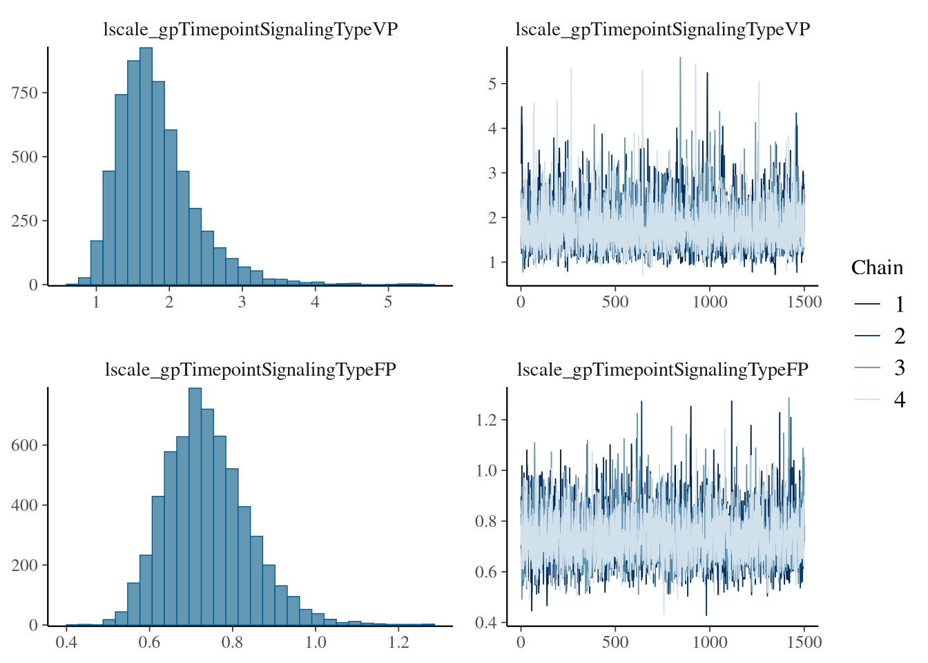
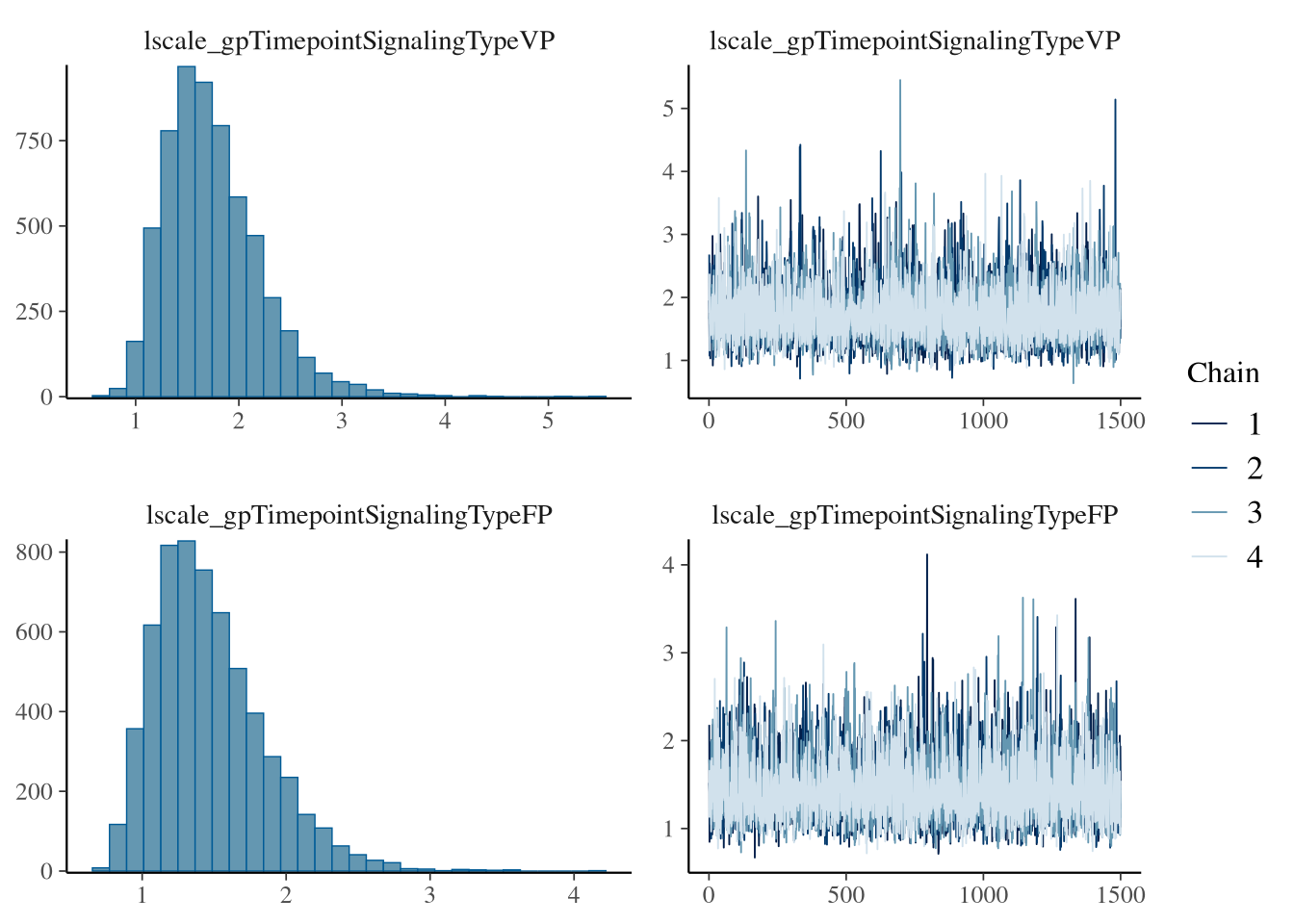
## lscale(gpTimepointSignalingTypeNP) 1.54 0.47 0.92 2.70 1.00 3729 3398
## lscale(gpTimepointSignalingTypeVP) 1.82 0.53 1.06 3.10 1.00 6116 3805
## lscale(gpTimepointSignalingTypeFP) 0.74 0.10 0.57 0.96 1.00 4236 3871
##
## Regression Coefficients:
## Estimate Est.Error l-95% CI u-95% CI Rhat Bulk_ESS Tail_ESS
## Intercept -0.10 0.19 -0.49 0.24 1.00 1893 2985
##
## Draws were sampled using sample(hmc). For each parameter, Bulk_ESS
## and Tail_ESS are effective sample size measures, and Rhat is the potential
## scale reduction factor on split chains (at convergence, Rhat = 1).Model diagnostics
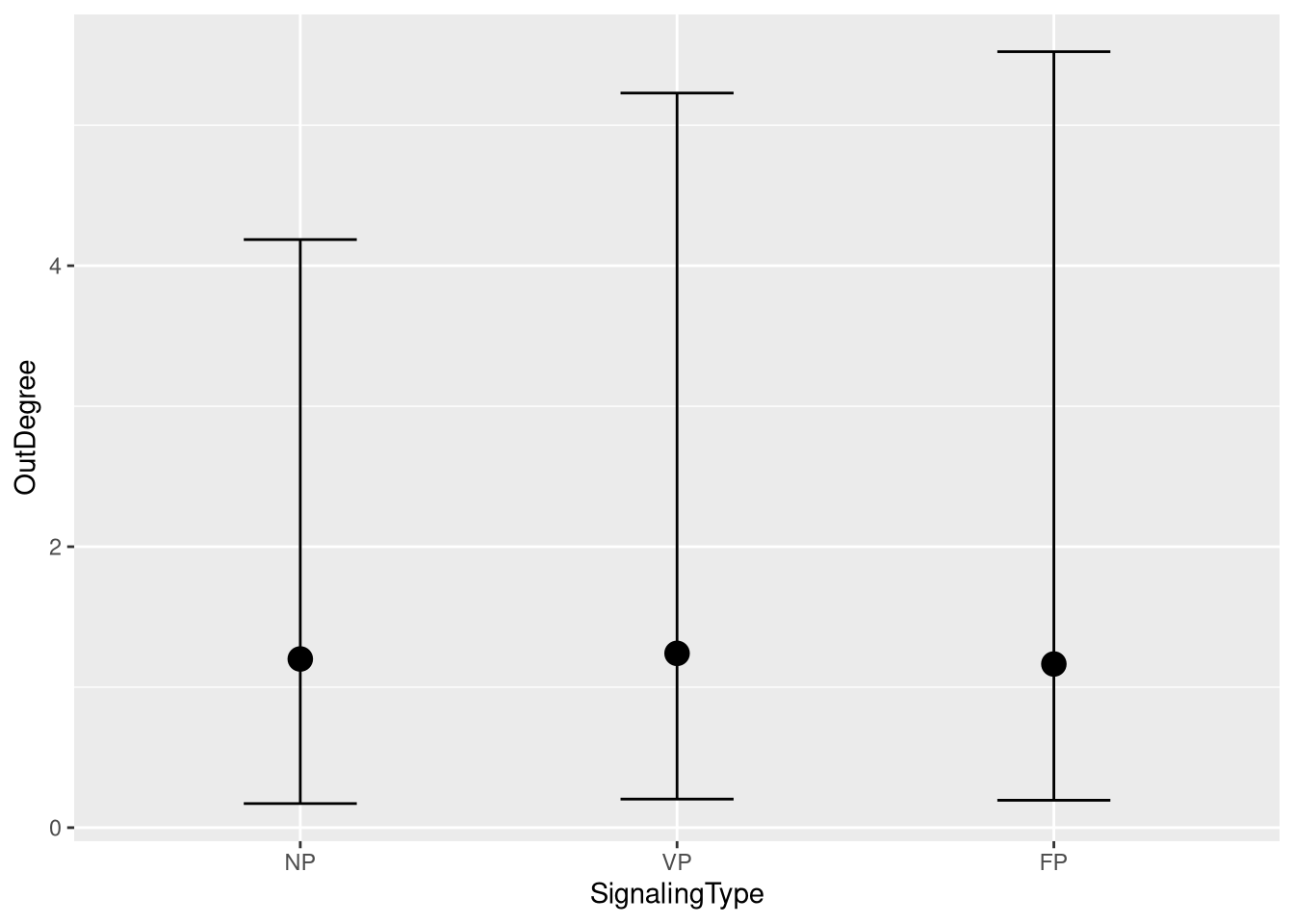
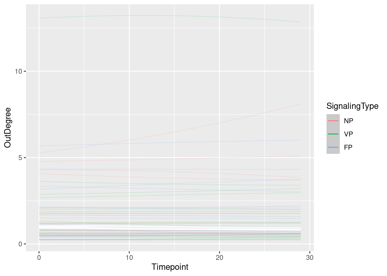
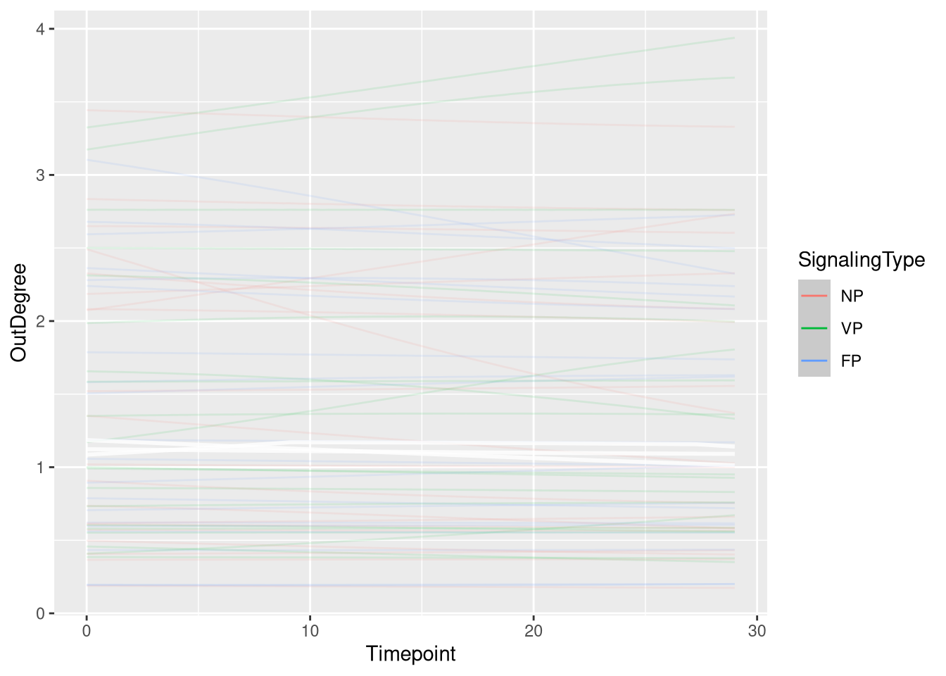
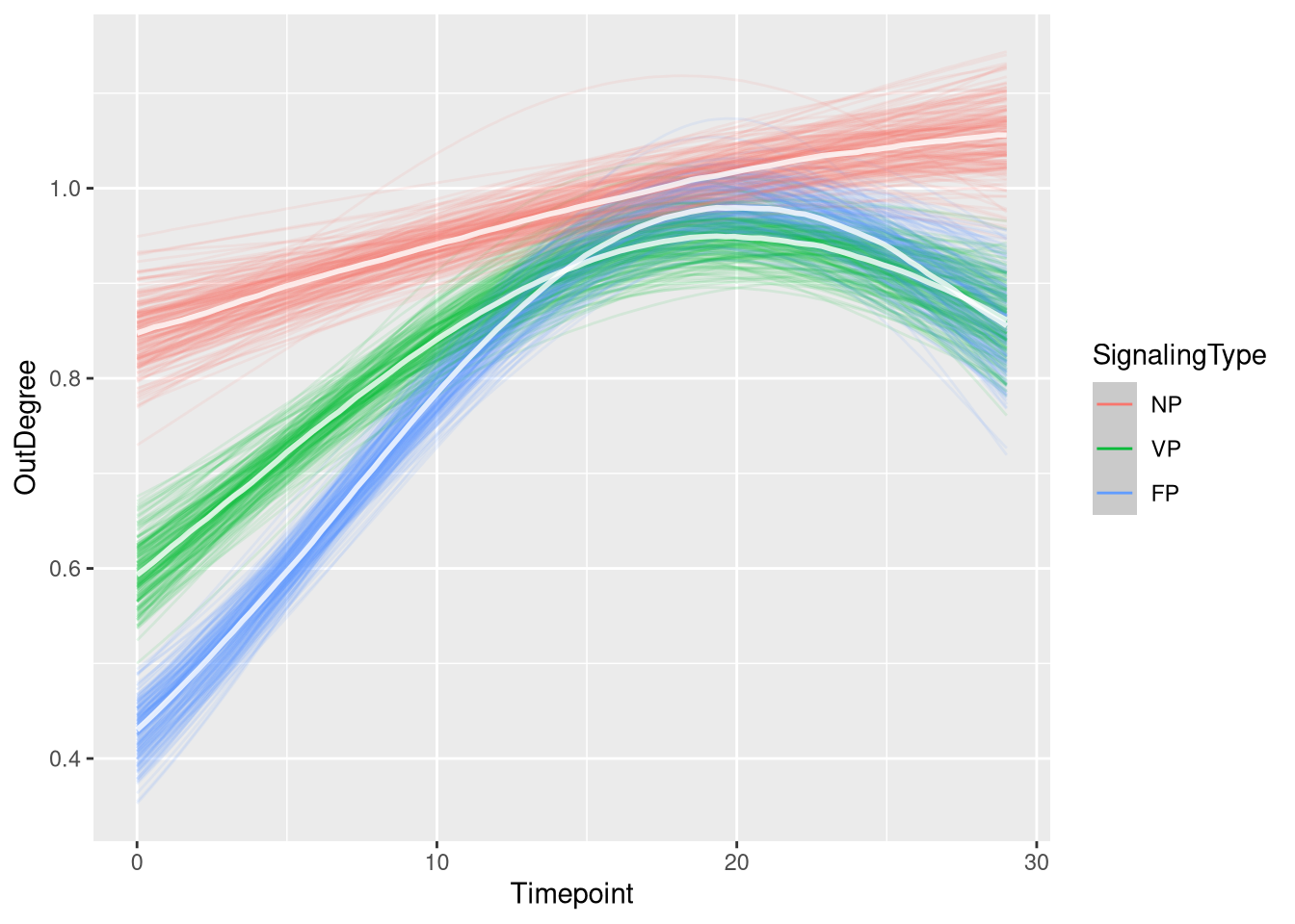
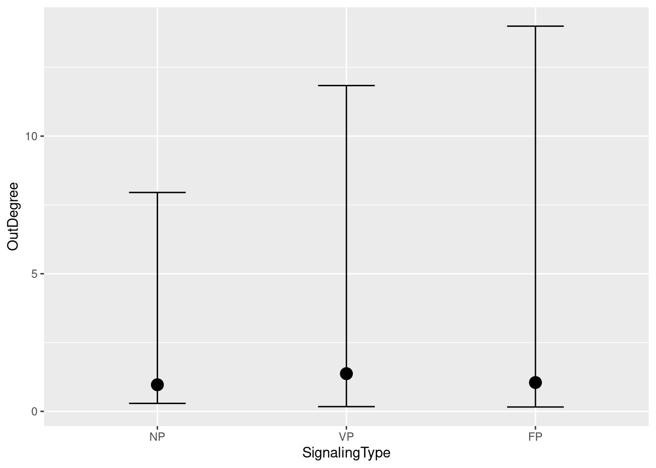
m.events.f.OutDegree.me <- conditional_effects(m.events.f.OutDegree.fit, ndraws = 200, spaghetti = TRUE)
plot(m.events.f.OutDegree.me, ask = FALSE, points = F)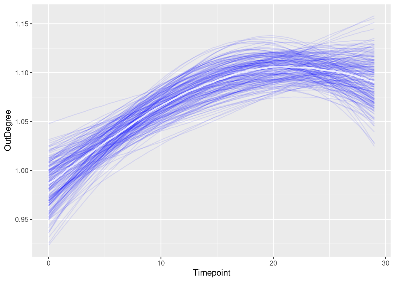
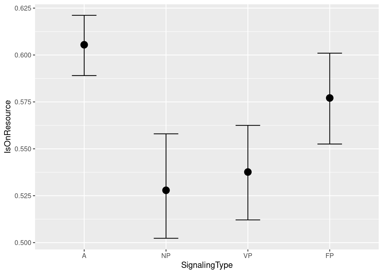
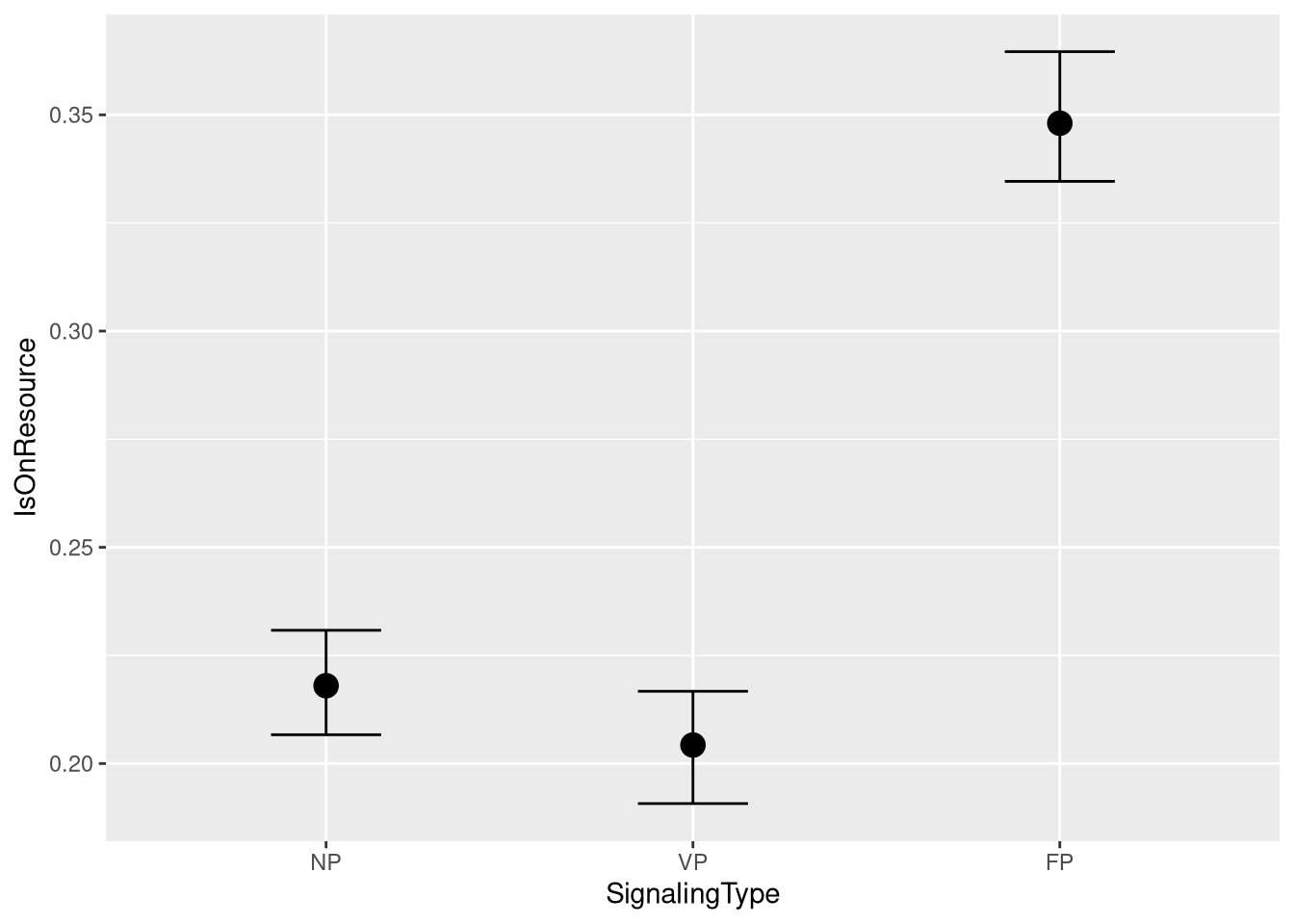
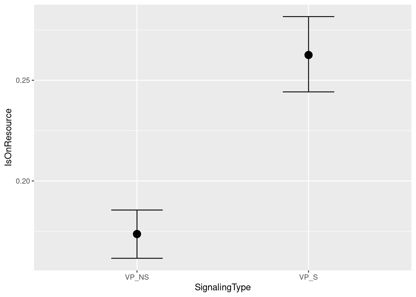
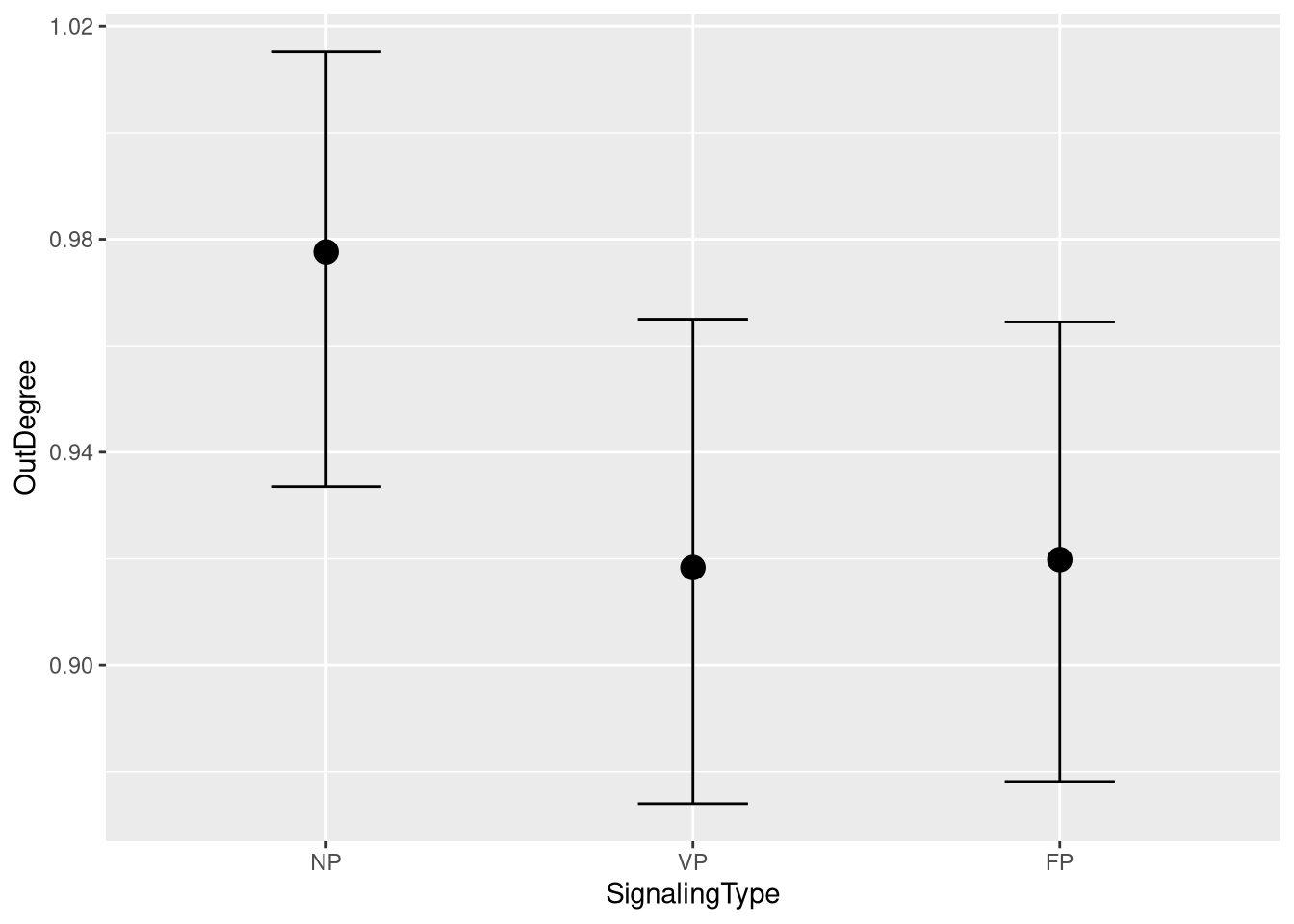
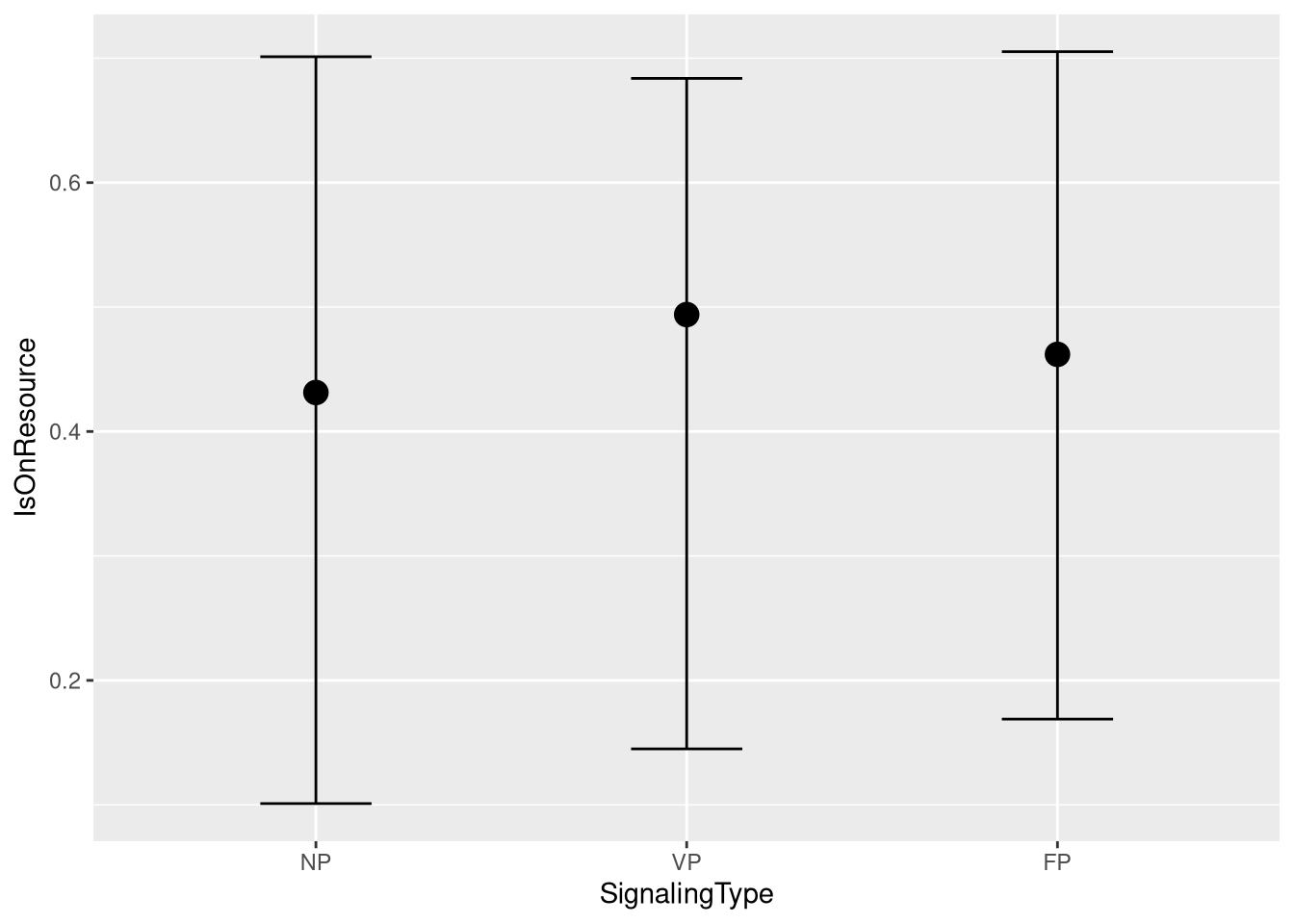
Statistical Comparisons
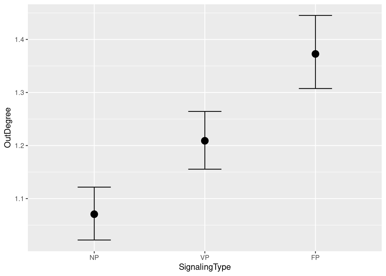
m.events.f.OutDegree.fit %>%
  emmeans(~ SignalingType,
          at = list(Timepoint = 10),
          epred = TRUE,
          type = "response") %>%
  contrast(method = "revpairwise", simple = "each", combine = TRUE) %>%
  gather_emmeans_draws() %>%
  mean_hdci(.width = 0.9) %>%
  mutate(.value = round(.value, 2), .lower = round(.lower, 2), .upper = round(.upper, 2)) %>%
  kable("html", digits = 2) %>%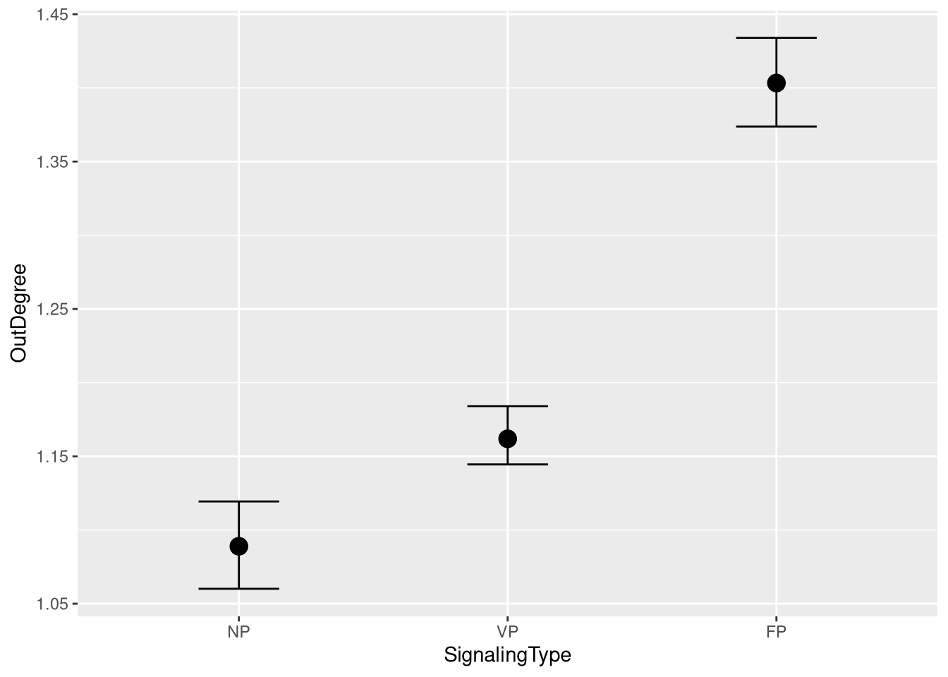
kable_classic(full_width = T, position = "center")| contrast | .value | .lower | .upper | .width | .point | .interval |
|---|---|---|---|---|---|---|
| FP - NP | 0.32 | 0.29 | 0.36 | 0.9 | mean | hdci |
| FP - VP | 0.27 | 0.23 | 0.30 | 0.9 | mean | hdci |
| VP - NP | 0.06 | 0.03 | 0.08 | 0.9 | mean | hdci |
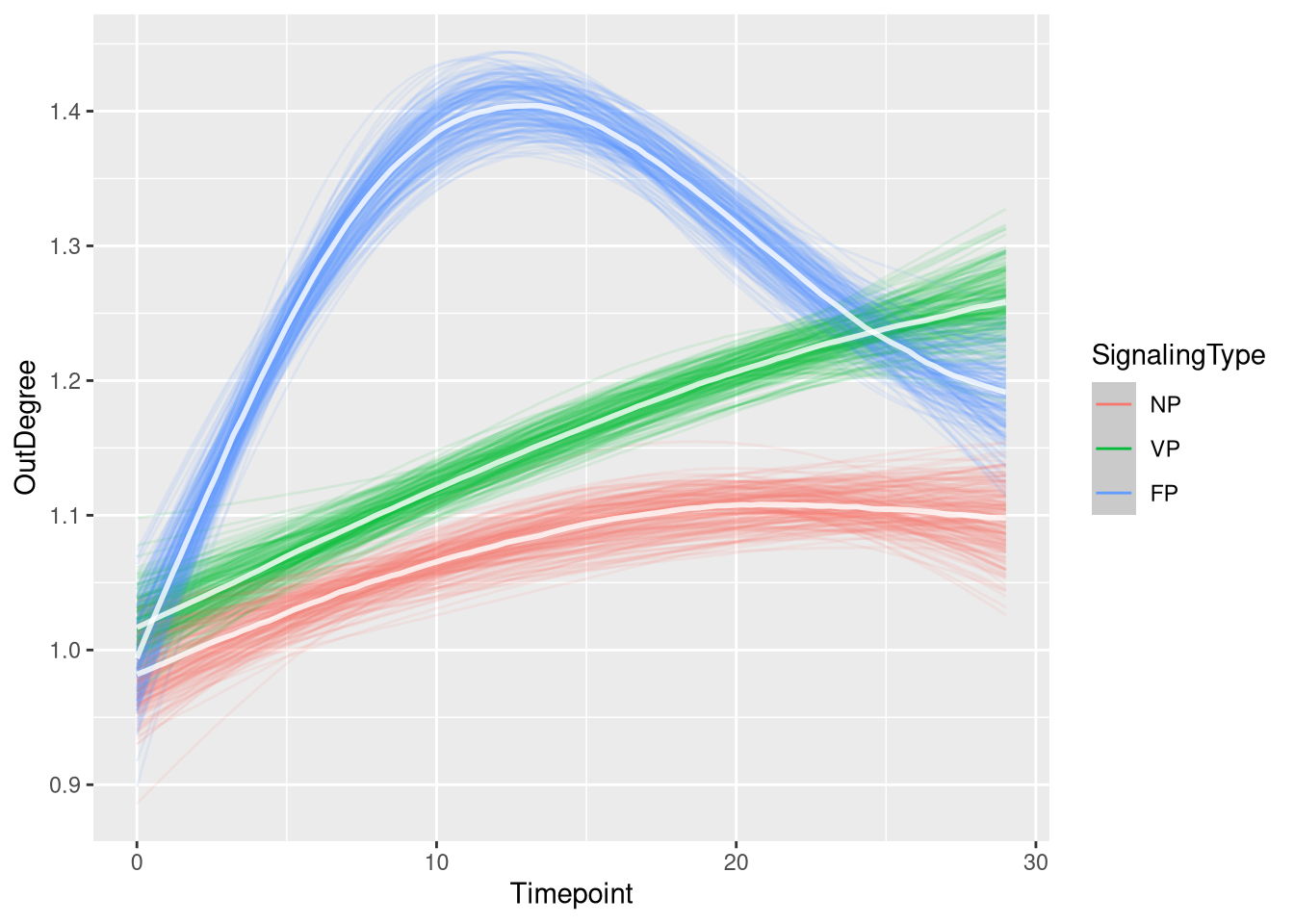
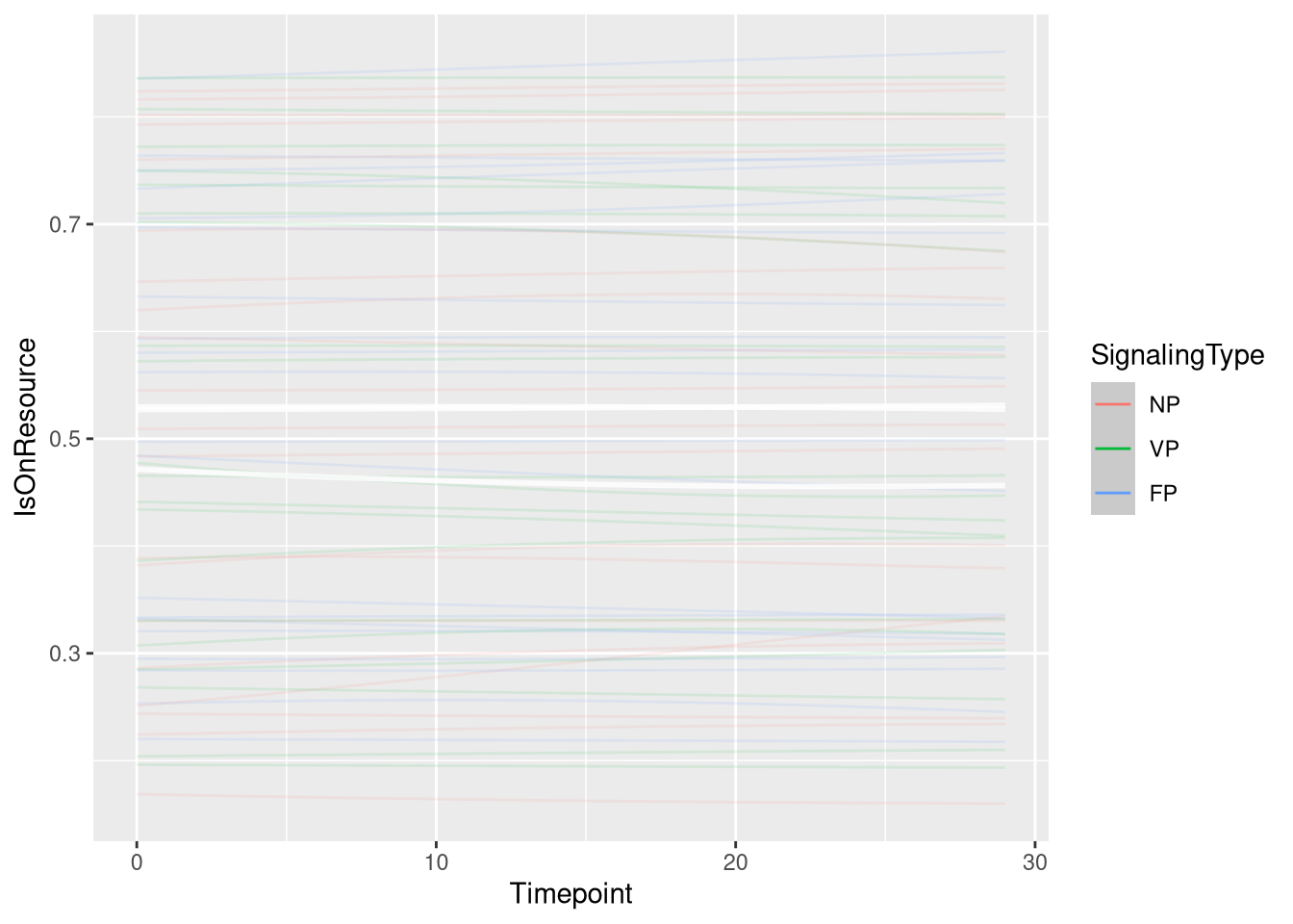
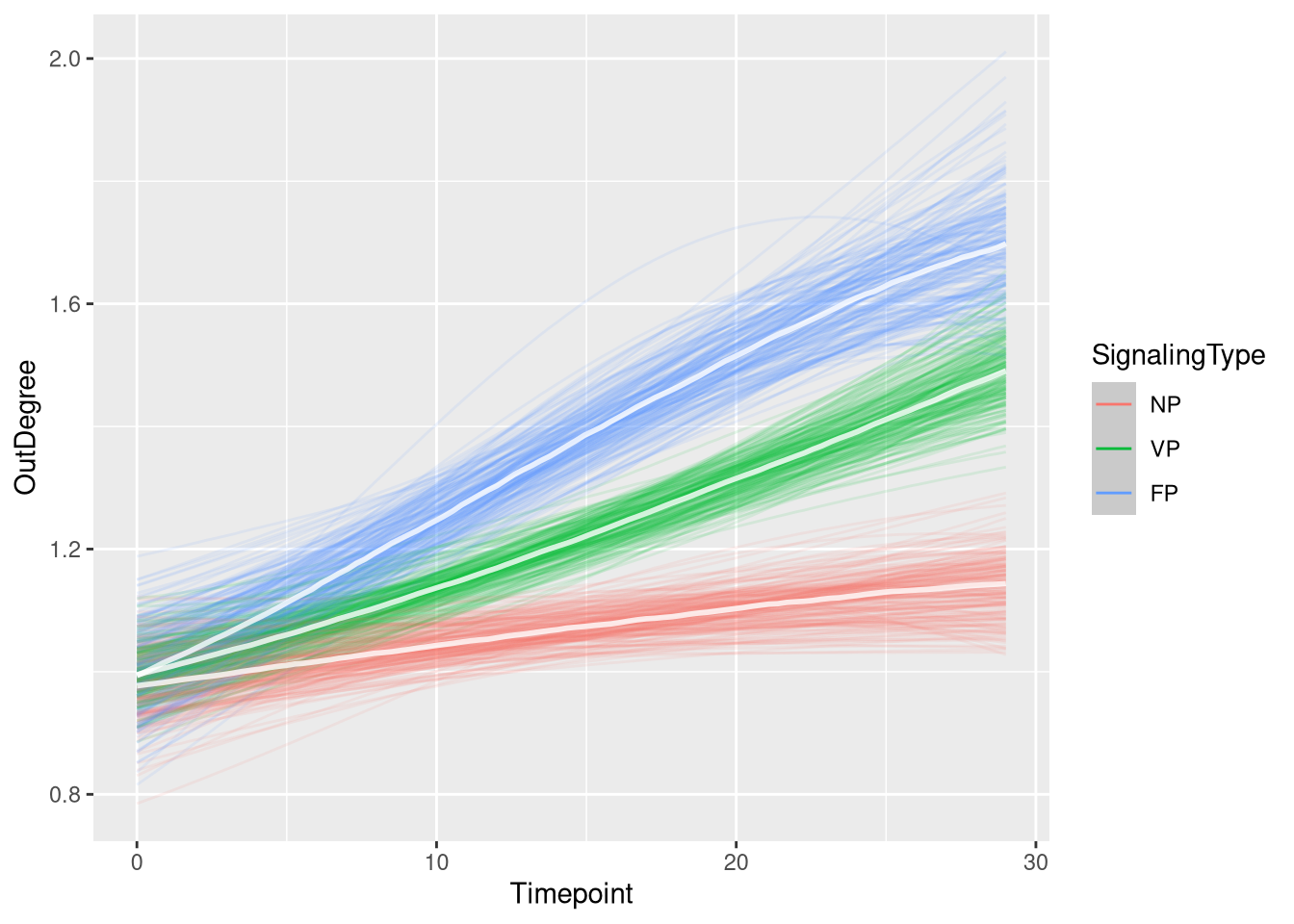
Figure
m.events.f.OutDegree.draws <- m.events.f.OutDegree.data %>%
mutate(SignalingType = factor(SignalingType, levels = c('NP', 'VP', 'FP'))) %>%
data_grid(Timepoint, SignalingType) %>%
tidybayes::add_epred_draws(m.events.f.OutDegree.fit, allow_new_levels = TRUE,
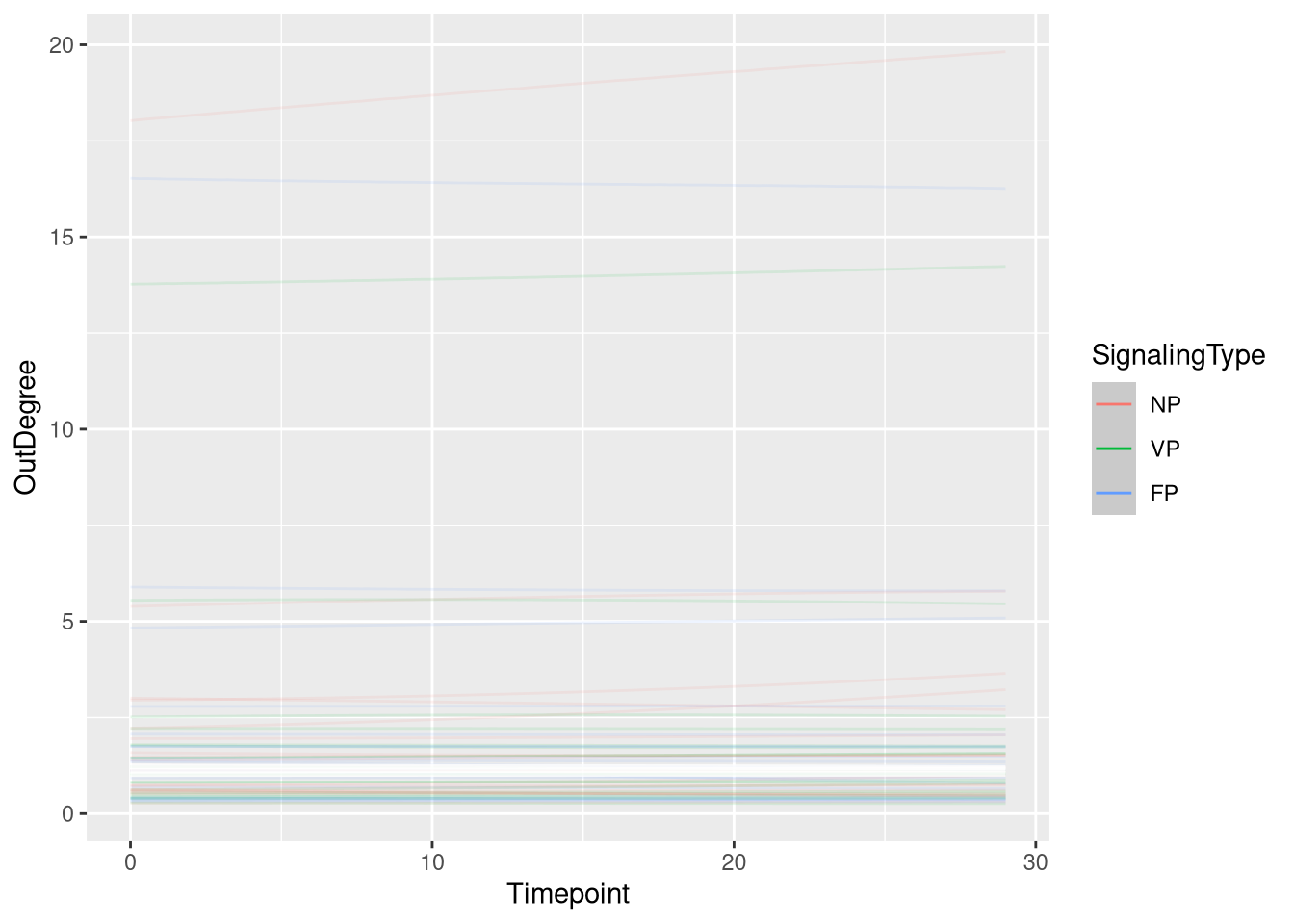
re_formula = m.events.f.OutDegree.formula)events_fast_outdegree_fig <- m.events.f.OutDegree.draws %>%
ggplot(aes(x = Timepoint, y = .epred, fill = SignalingType, color = SignalingType)) + # , group = SignalingType
stat_lineribbon(aes(group = paste(group, ...width..)), .width = c(.9), alpha = 1/2) +
scale_color_manual(breaks = c('NP', 'VP', 'FP'),
aesthetics = c("colour", "fill"),
values = c("#DF536B", "#61D04F", "#2297E6"),
guide = guide_legend(
title = "Signaling",
)
) +
# theme_nice(legend.pos = 'top') +
theme_clean() +
panel_border() +
theme(legend.position = "none") +
scale_x_continuous(
limits = c(0, 30),
expand = expansion(mult = c(0, 0))
) +
labs(x = "Time [s]",
y = "Out Degree")
events_fast_outdegree_fig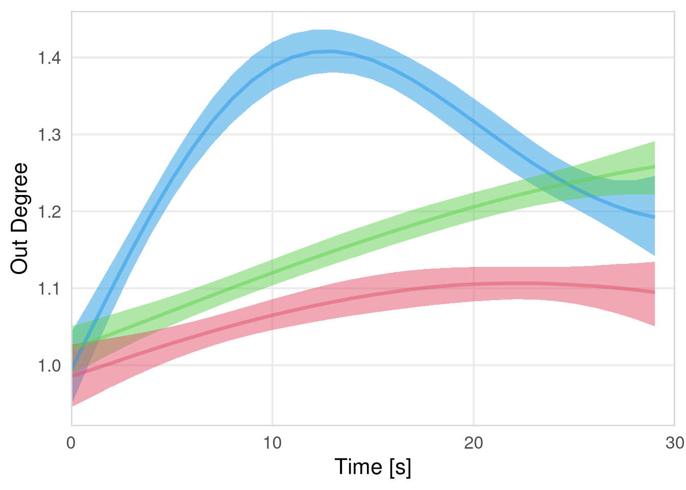
Out degree (Discoverer)
m.events.f.OutDegree.Discoverer.data  <- resource_discoveries_data %>%
  filter(ResourceSpeed == 'fast', SignalingType != 'A', PlayerOrderCat == 'first') %>%
  filter(((Timepoint * 10) %% 10 == 0))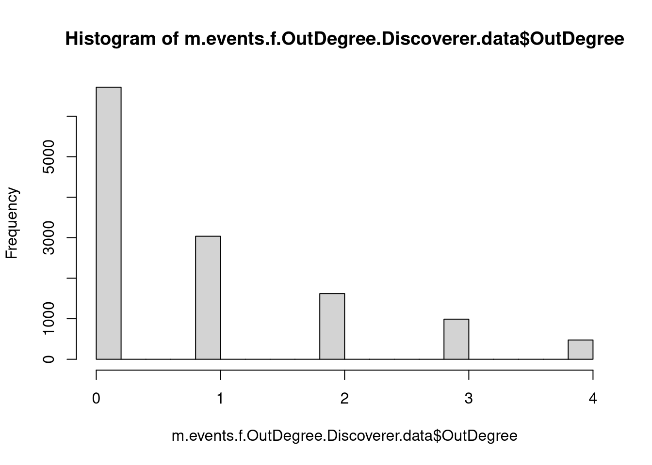
m.events.f.OutDegree.Discoverer.formula <- brmsformula(
  OutDegree ~ gp(Timepoint, by = SignalingType),
  family = poisson(link = "log")
  )
m.events.f.OutDegree.Discoverer.priors <-
prior(normal(0, 1), class = "Intercept") +
prior(inv_gamma(10, 20), class = "lscale", coef = "gpTimepointSignalingTypeFP") +
prior(inv_gamma(10, 20), class = "lscale", coef = "gpTimepointSignalingTypeNP") +
prior(inv_gamma(10, 20), class = "lscale", coef = "gpTimepointSignalingTypeVP") +
prior(normal(0, 0.25), class = "sdgp", lb = 0)Prior predictive checks
m.events.f.OutDegree.Discoverer.fit_prior <- brm(
  formula = m.events.f.OutDegree.Discoverer.formula,
  family = poisson(link = "log"),
  prior = m.events.f.OutDegree.Discoverer.priors,
  m.events.f.OutDegree.Discoverer.data,
  chains  = 4,
  cores   = 4,
  seed    = 42,
  iter    = 2000,
  file = paste0(fits_path, 'resource_discoveries_fast_out_degree_discoverer_prior.rds'),
  backend = "cmdstanr",
  threads = threading(100),
  control = list(adapt_delta = 0.95),
  save_pars = save_pars(all = TRUE),
  sample_prior = "only"
)plot(conditional_effects(m.events.f.OutDegree.Discoverer.fit_prior, ndraws = 20, spaghetti = TRUE), points = F, ask = F)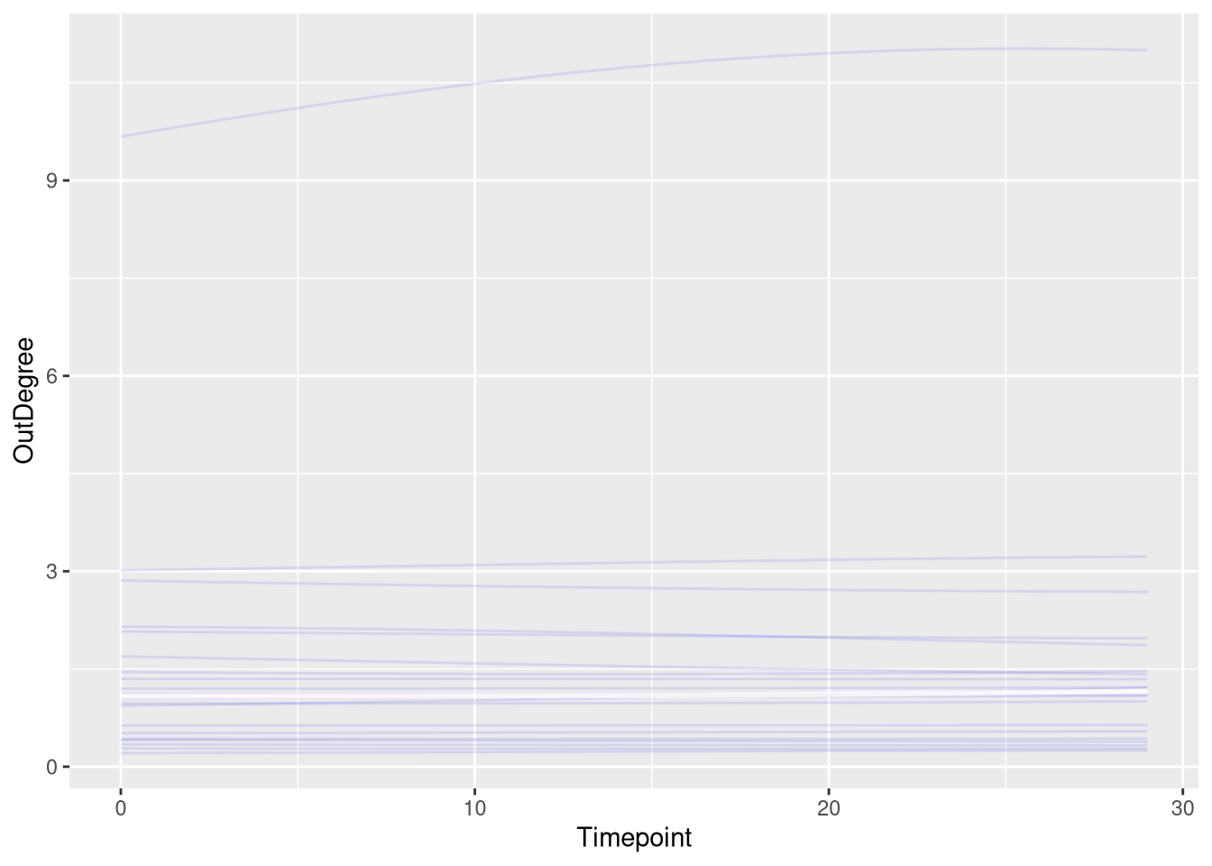
Model fitting
m.events.f.OutDegree.Discoverer.fit <- brm(
  formula = m.events.f.OutDegree.Discoverer.formula,
  prior   = m.events.f.OutDegree.Discoverer.priors,
  data    = m.events.f.OutDegree.Discoverer.data ,
  chains = 4,
  cores = 4,
  seed = 42,
  warmup = 500,
  iter = 2000,
  file = paste0(fits_path, 'resource_discoveries_fast_out_degree_discoverer.rds'),
  backend = "cmdstanr",
  threads = threading(100),
  control = list(adapt_delta = 0.95),
  save_pars = save_pars(all = TRUE)
)## Family: poisson
## Links: mu = log
## Formula: OutDegree ~ gp(Timepoint, by = SignalingType)
## Data: m.events.f.OutDegree.Discoverer.data (Number of observations: 12840)
## Draws: 4 chains, each with iter = 2000; warmup = 500; thin = 1;
## total post-warmup draws = 6000
##
## Gaussian Process Hyperparameters:
## Estimate Est.Error l-95% CI u-95% CI Rhat Bulk_ESS Tail_ESS
## sdgp(gpTimepointSignalingTypeNP) 0.40 0.14 0.17 0.71 1.00 4617 3563
## sdgp(gpTimepointSignalingTypeVP) 0.56 0.15 0.30 0.87 1.00 5613 4270
## sdgp(gpTimepointSignalingTypeFP) 0.67 0.15 0.41 0.99 1.00 5527 3415
## lscale(gpTimepointSignalingTypeNP) 1.83 0.53 1.06 3.12 1.00 8727 4320
## lscale(gpTimepointSignalingTypeVP) 1.00 0.17 0.71 1.37 1.00 6807 4902
## lscale(gpTimepointSignalingTypeFP) 0.86 0.13 0.63 1.13 1.00 6645 4521
##
## Regression Coefficients:
## Estimate Est.Error l-95% CI u-95% CI Rhat Bulk_ESS Tail_ESS
## Intercept -0.54 0.27 -1.09 -0.04 1.00 2856 3232
##
## Draws were sampled using sample(hmc). For each parameter, Bulk_ESS
## and Tail_ESS are effective sample size measures, and Rhat is the potential
## scale reduction factor on split chains (at convergence, Rhat = 1).Model diagnostics
m.events.f.OutDegree.Discoverer.me <- conditional_effects(m.events.f.OutDegree.Discoverer.fit, ndraws = 200, spaghetti = TRUE)
plot(m.events.f.OutDegree.Discoverer.me, ask = FALSE, points = F)
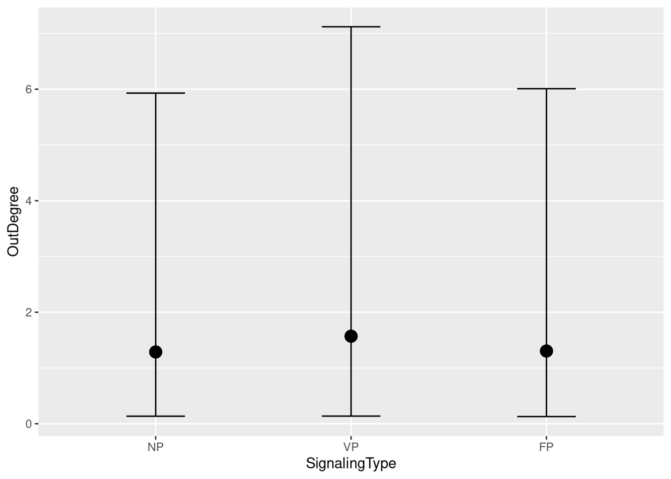
Statistical Comparisons
m.events.f.OutDegree.Discoverer.fit %>%
  emmeans(~ SignalingType,
          at = list(Timepoint = 10),
          epred = TRUE,
          type = "response") %>%
  contrast(method = "revpairwise", simple = "each", combine = TRUE) %>%
  gather_emmeans_draws() %>%
  mean_hdci(.width = 0.9) %>%
  mutate(.value = round(.value, 2), .lower = round(.lower, 2), .upper = round(.upper, 2)) %>%
  kable("html", digits = 2) %>%
kable_classic(full_width = T, position = "center")| contrast | .value | .lower | .upper | .width | .point | .interval |
|---|---|---|---|---|---|---|
| FP - NP | -0.15 | -0.20 | -0.11 | 0.9 | mean | hdci |
| FP - VP | -0.06 | -0.11 | -0.01 | 0.9 | mean | hdci |
| VP - NP | -0.10 | -0.15 | -0.06 | 0.9 | mean | hdci |
Figure
m.events.f.OutDegree.Discoverer.draws <- m.events.f.OutDegree.Discoverer.data  %>%
  mutate(SignalingType = factor(SignalingType, levels = c('NP', 'VP', 'FP'))) %>%
  data_grid(Timepoint, SignalingType) %>%
  tidybayes::add_epred_draws(m.events.f.OutDegree.Discoverer.fit, allow_new_levels = TRUE,
                             re_formula = m.events.f.OutDegree.Discoverer.formula)
events_fast_outdegree_discoverer_fig <- m.events.f.OutDegree.Discoverer.draws %>%
ggplot(aes(x = Timepoint, y = .epred, fill = SignalingType, color = SignalingType)) +
stat_lineribbon(aes(group = paste(group, ...width..)), .width = c(.9), alpha = 1/2) +
scale_color_manual(breaks = c('NP', 'VP', 'FP'),
aesthetics = c("colour", "fill"),
values = c("#DF536B", "#61D04F", "#2297E6"),
guide = guide_legend(
title = "Signaling",
)
) +
# theme_nice(legend.pos = 'top') +
theme_clean() +
panel_border() +
theme(legend.position = "none") +
scale_x_continuous(
limits = c(0, 30),
expand = expansion(mult = c(0, 0))
) +
labs(x = "Time [s]",
y = "Out Degree")
events_fast_outdegree_discoverer_fig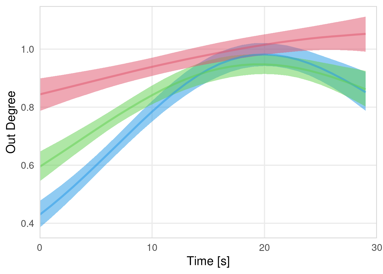
Out degree VP
m.events.f.OutDegree.VP.data  <- resource_discoveries_data_vp %>%
  filter(ResourceSpeed == 'fast', PlayerOrderCat == 'others') %>%
  filter(((Timepoint * 10) %% 10 == 0))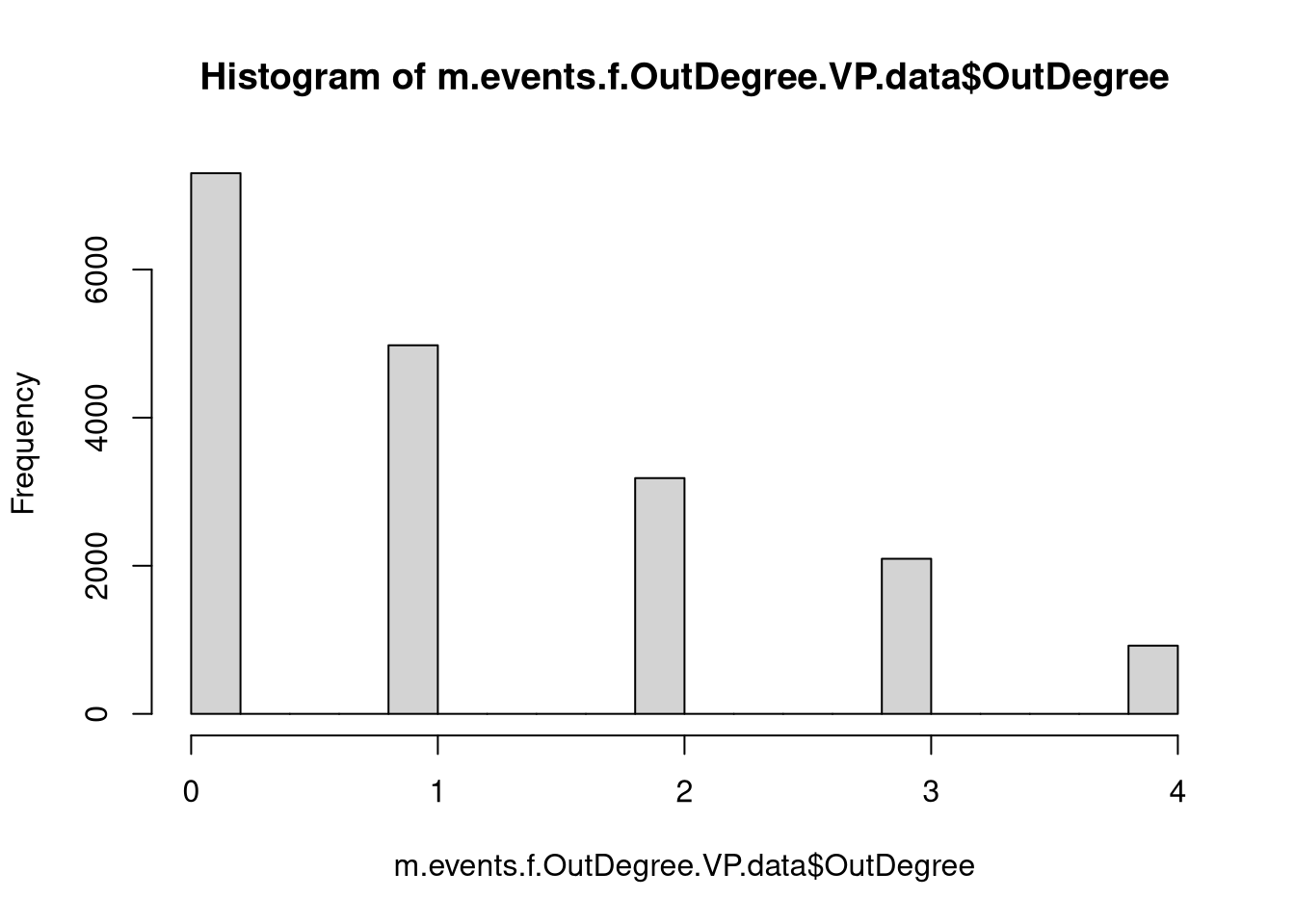
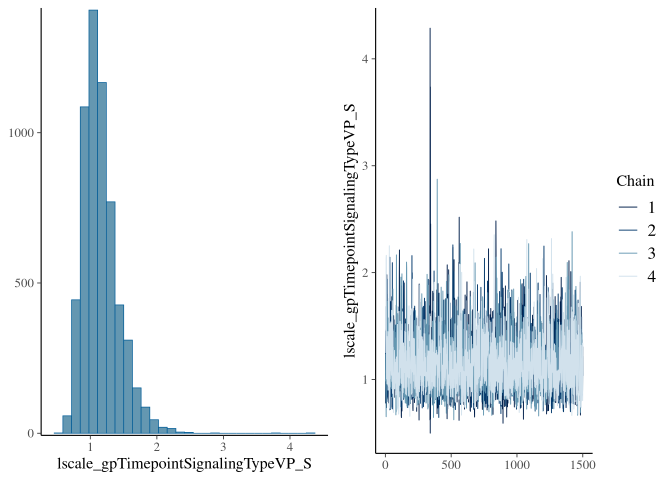
m.events.f.OutDegree.VP.formula <- brmsformula(
  OutDegree ~ 1 + gp(Timepoint, by = SignalingType),
  family = negbinomial()
  )
m.events.f.OutDegree.VP.priors <-
prior(normal(0, 1), class = "Intercept") +
prior(inv_gamma(10, 20), class = "lscale", coef = "gpTimepointSignalingTypeVP_NS") +
prior(inv_gamma(10, 20), class = "lscale", coef = "gpTimepointSignalingTypeVP_S") +
prior(normal(0, 0.1), class = "sdgp", lb = 0)Prior predictive checks
m.events.f.OutDegree.VP.fit_prior <- brm(
  formula = m.events.f.OutDegree.VP.formula,
  prior   = m.events.f.OutDegree.VP.priors,
  data    = m.events.f.OutDegree.VP.data,
  chains  = 4,
  cores   = 4,
  seed    = 42,
  iter    = 2000,
  file = paste0(fits_path, 'resource_discoveries_fast_out_degree_vp_prior.rds'),
  backend = "cmdstanr",
  threads = threading(100),
  control = list(adapt_delta = 0.95),
  save_pars = save_pars(all = TRUE),
  sample_prior = "only"
)plot(conditional_effects(m.events.f.OutDegree.VP.fit_prior, ndraws = 20, spaghetti = TRUE), points = F, ask = F)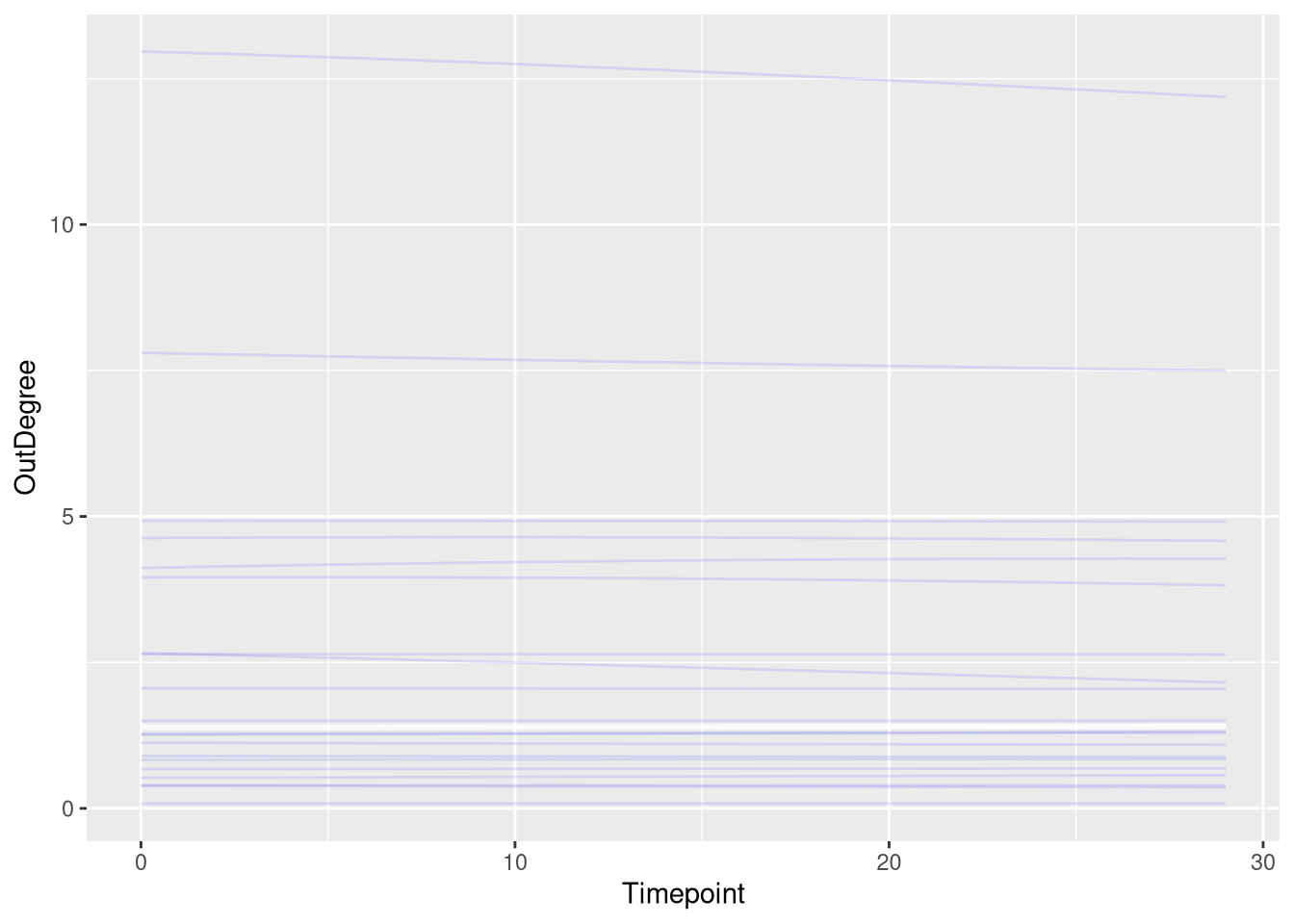
Model fitting
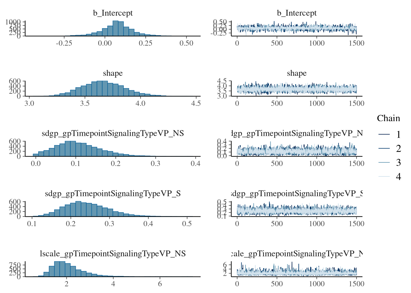
m.events.f.OutDegree.VP.fit <- brm(
  formula = m.events.f.OutDegree.VP.formula,
  prior   = m.events.f.OutDegree.VP.priors,
  data    = m.events.f.OutDegree.VP.data,
  chains = 4,
  cores = 4,
  seed = 42,
  warmup = 500,
  iter = 2000,
  file = paste0(fits_path, 'resource_discoveries_fast_out_degree_vp.rds'),
  backend = "cmdstanr",
  threads = threading(100),
  control = list(adapt_delta = 0.95),
  save_pars = save_pars(all = TRUE)
)## Family: negbinomial
## Links: mu = log; shape = identity
## Formula: OutDegree ~ 1 + gp(Timepoint, by = SignalingType)
## Data: m.events.f.OutDegree.VP.data (Number of observations: 18480)
## Draws: 4 chains, each with iter = 2000; warmup = 500; thin = 1;
## total post-warmup draws = 6000
##
## Gaussian Process Hyperparameters:
## Estimate Est.Error l-95% CI u-95% CI Rhat Bulk_ESS Tail_ESS
## sdgp(gpTimepointSignalingTypeVP_NS) 0.11 0.06 0.01 0.23 1.00 2074 1367
## sdgp(gpTimepointSignalingTypeVP_S) 0.24 0.06 0.14 0.36 1.00 4938 3879
## lscale(gpTimepointSignalingTypeVP_NS) 2.06 0.67 1.13 3.70 1.00 7445 4453
## lscale(gpTimepointSignalingTypeVP_S) 1.16 0.27 0.76 1.80 1.00 5301 4197
##
## Regression Coefficients:
## Estimate Est.Error l-95% CI u-95% CI Rhat Bulk_ESS Tail_ESS
## Intercept 0.07 0.09 -0.13 0.27 1.00 2342 2566
##
## Further Distributional Parameters:
## Estimate Est.Error l-95% CI u-95% CI Rhat Bulk_ESS Tail_ESS
## shape 3.66 0.19 3.31 4.06 1.00 9055 4160
##
## Draws were sampled using sample(hmc). For each parameter, Bulk_ESS
## and Tail_ESS are effective sample size measures, and Rhat is the potential
## scale reduction factor on split chains (at convergence, Rhat = 1).Model diagnostics
m.events.f.OutDegree.VP.me <- conditional_effects(m.events.f.OutDegree.VP.fit, ndraws = 200, spaghetti = TRUE)
plot(m.events.f.OutDegree.VP.me, ask = FALSE, points = F)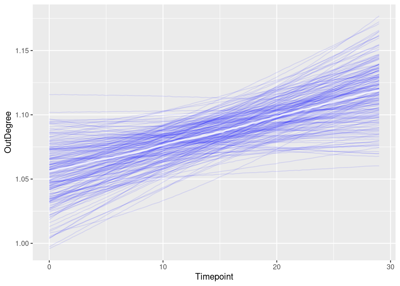
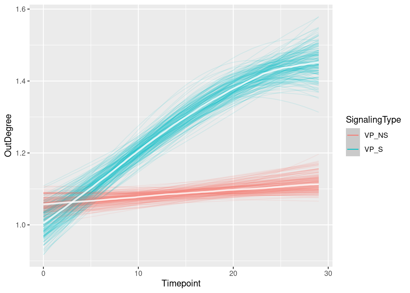
Figure
m.events.f.OutDegree.VP.draws <- m.events.f.OutDegree.VP.data %>%
mutate(SignalingType = factor(SignalingType, levels = c('VP_NS', 'VP_S'))) %>%
data_grid(Timepoint, SignalingType) %>%
tidybayes::add_epred_draws(m.events.f.OutDegree.VP.fit, allow_new_levels = TRUE,
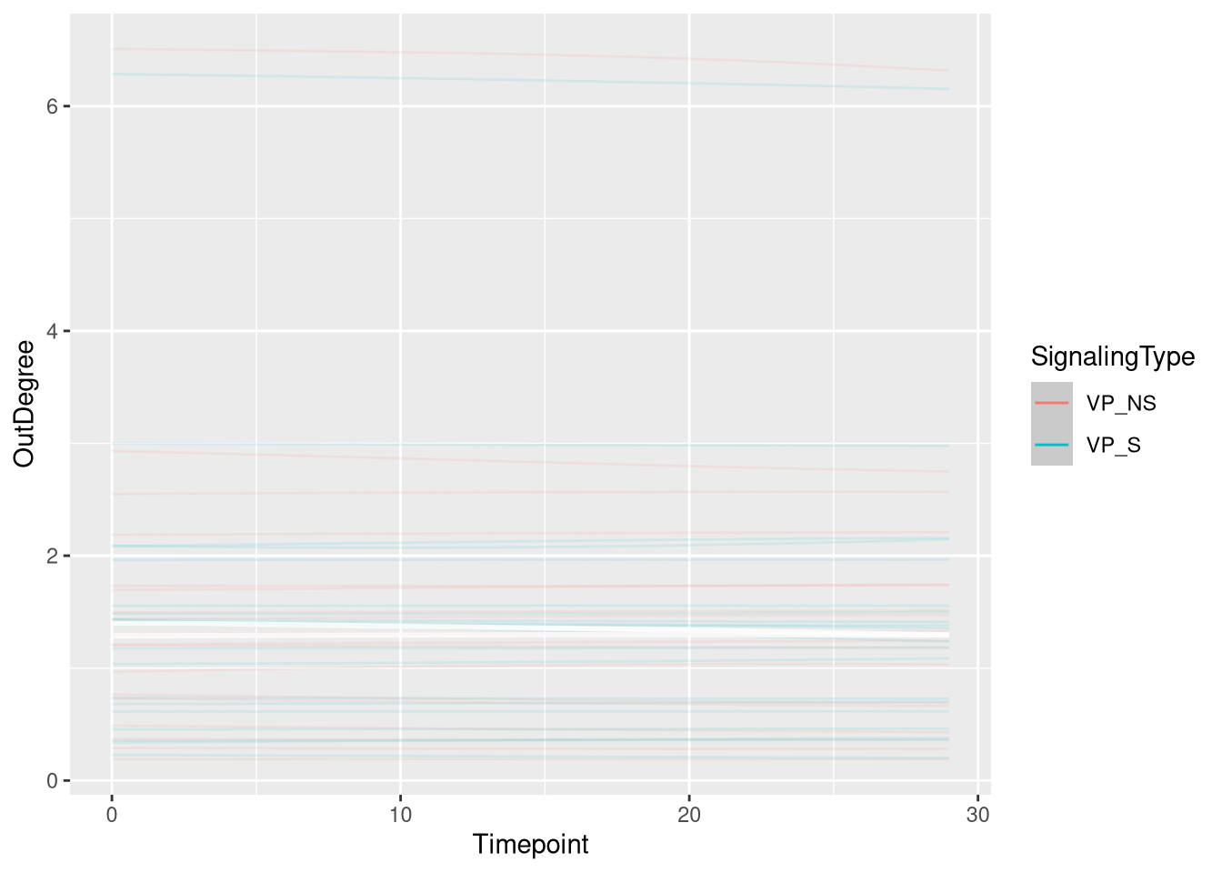
re_formula = m.events.f.OutDegree.VP.formula)events_fast_outdegree_vp_fig <- m.events.f.OutDegree.VP.draws %>%
ggplot(aes(x = Timepoint, y = .epred, fill = SignalingType, color = SignalingType)) +
stat_lineribbon(aes(group = paste(group, ...width..)), .width = c(.9), alpha = 1/2) +
theme_nice(legend.pos = 'none') +
scale_color_manual(breaks = c('VP_NS', 'VP_S'),
aesthetics = c("colour", "fill"),
values = c("#000000", "#DF536B"),
guide = guide_legend(
title = "Signaling",
)
) +
theme_clean() +
panel_border() +
theme(legend.position = "none") +
scale_x_continuous(
limits = c(0, 30),
expand = expansion(mult = c(0, 0))
) +
labs(x = "Time [s]",
y = "Out Degree")
events_fast_outdegree_vp_fig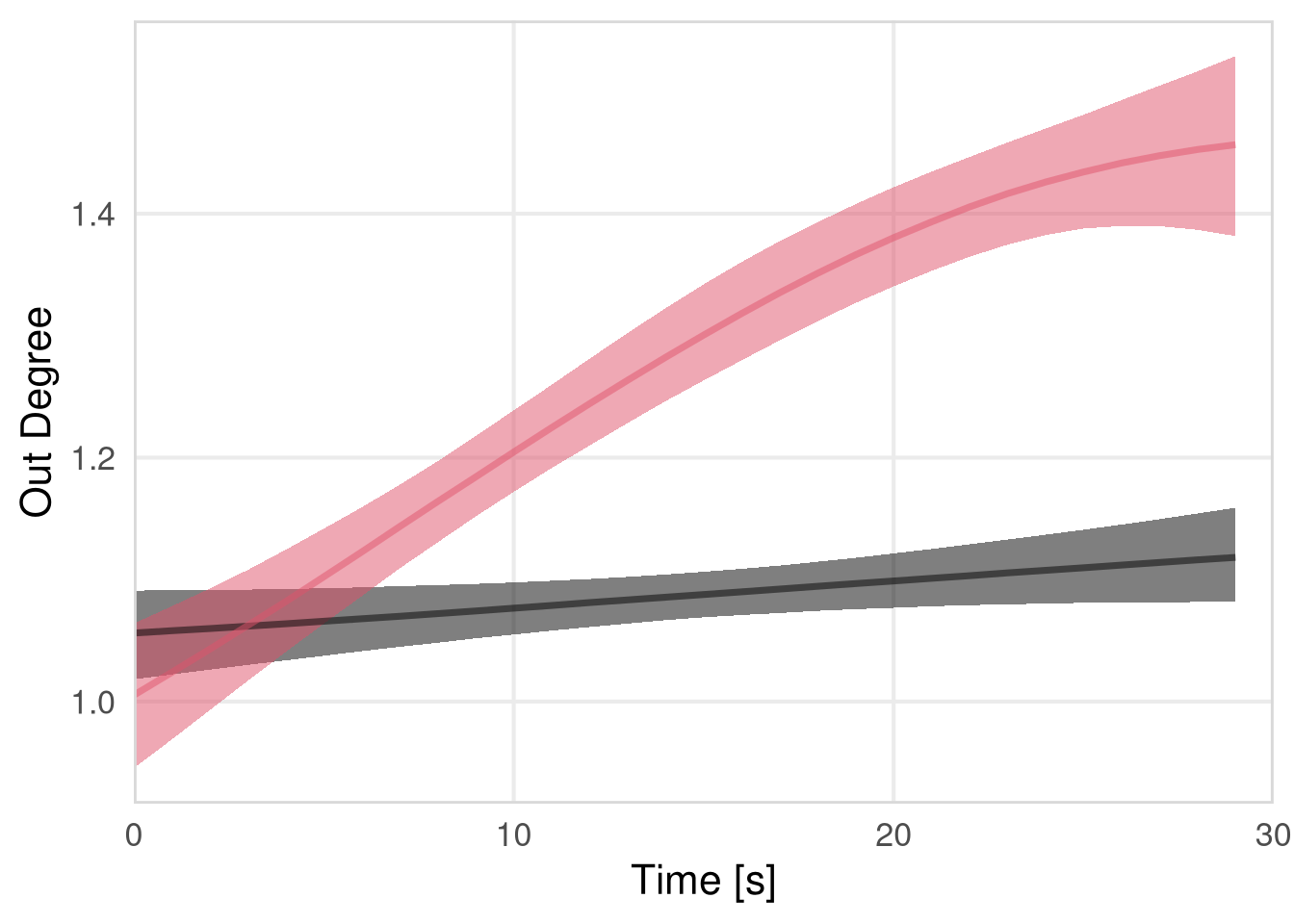
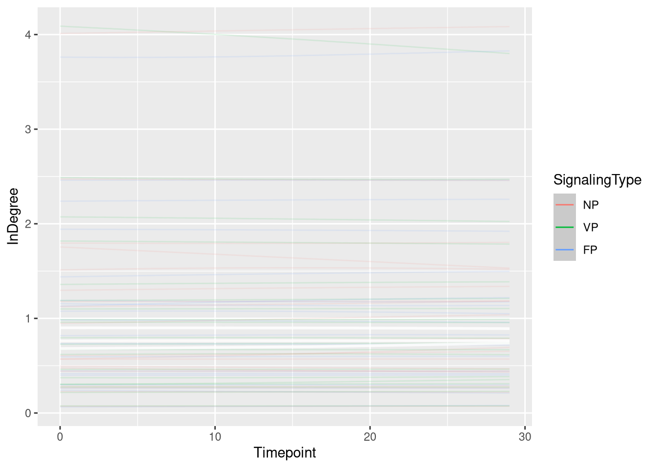
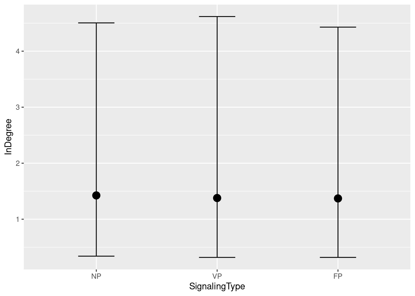
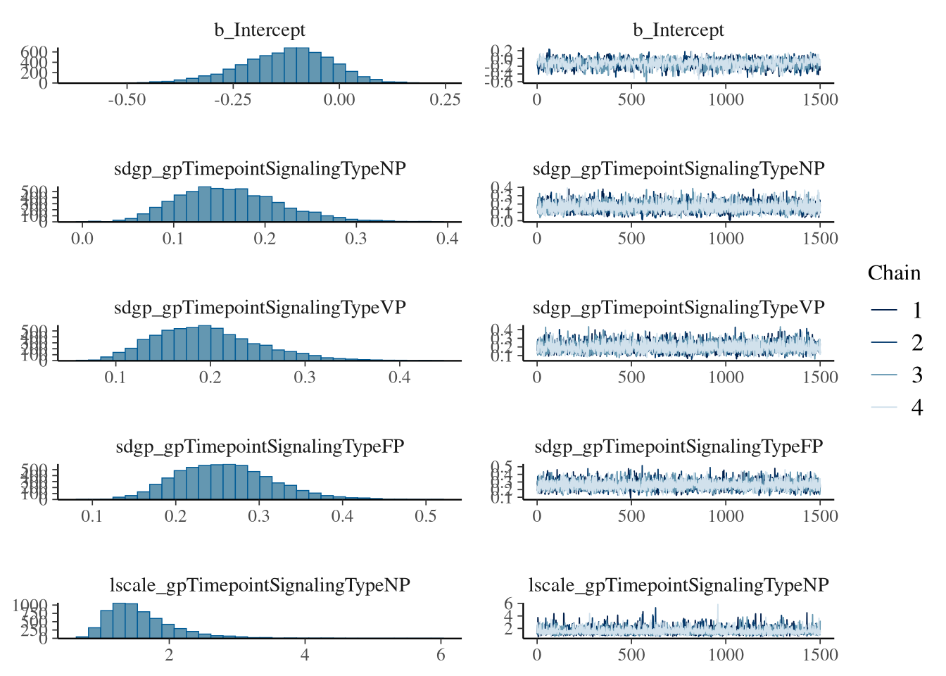
In degree
m.events.f.InDegree.data <- resource_discoveries_data %>%
  filter(ResourceSpeed == 'fast', SignalingType != 'A', PlayerOrderCat == 'first') %>%
  filter(((Timepoint * 10) %% 10 == 0))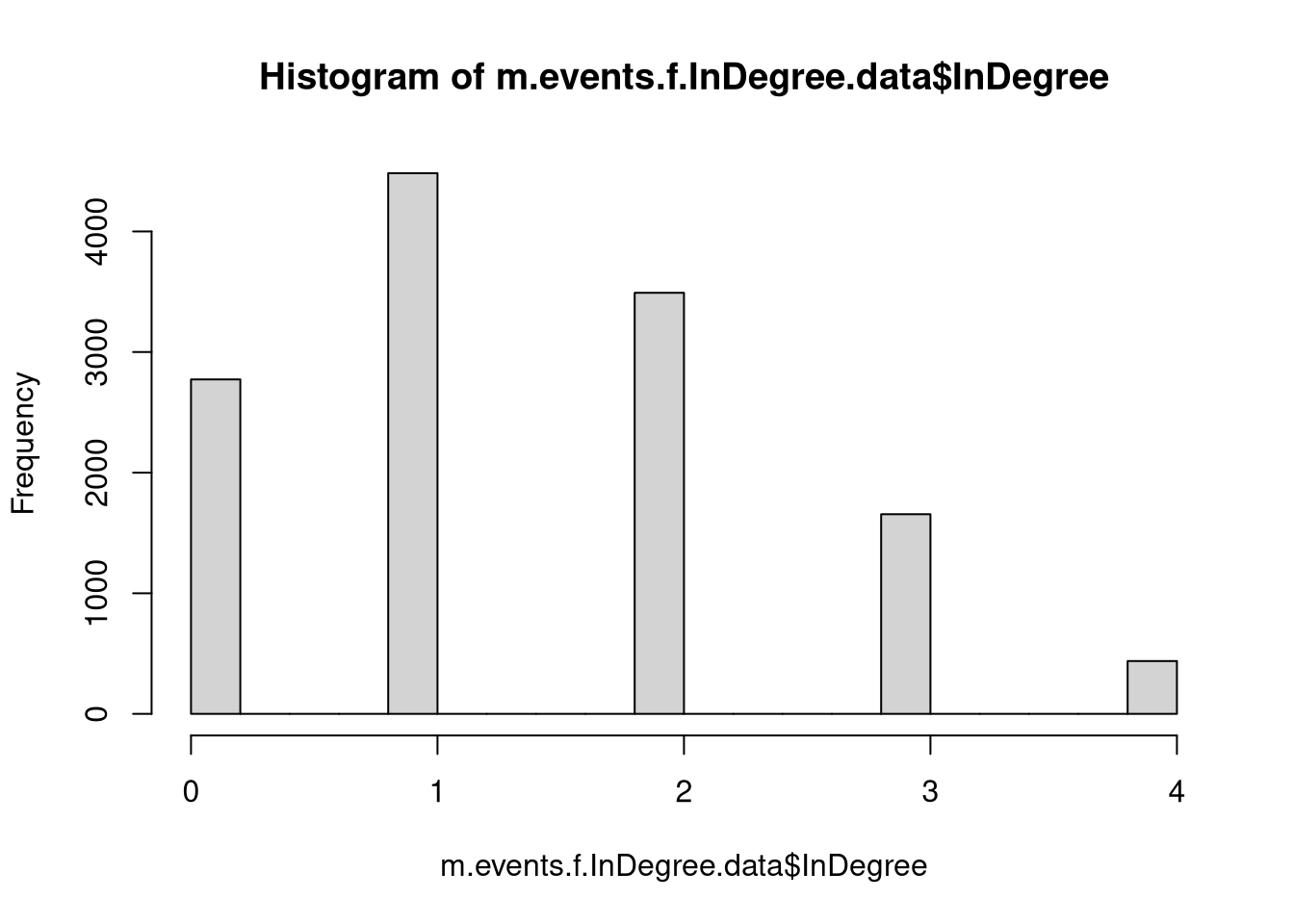
m.events.f.InDegree.formula <- brmsformula(
  InDegree ~ gp(Timepoint, by = SignalingType),
  family = poisson(link = "log")
  )
m.events.f.InDegree.priors <-
prior(normal(0, 1), class = "Intercept") +
prior(inv_gamma(10, 20), class = "lscale", coef = "gpTimepointSignalingTypeFP") +
prior(inv_gamma(10, 20), class = "lscale", coef = "gpTimepointSignalingTypeNP") +
prior(inv_gamma(10, 20), class = "lscale", coef = "gpTimepointSignalingTypeVP") +
prior(normal(0, 0.1), class = "sdgp", lb = 0)Prior predictive checks
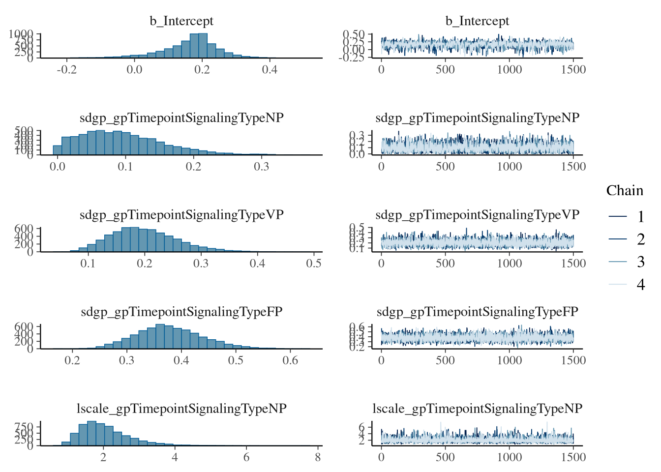
m.events.f.InDegree.fit_prior <- brm(
  formula = m.events.f.InDegree.formula,
  prior   = m.events.f.InDegree.priors,
  data    = m.events.f.InDegree.data,
  chains  = 4,
  cores   = 4,
  seed    = 42,
  iter    = 2000,
  file = paste0(fits_path, 'resource_discoveries_fast_in_degree_prior.rds'),
  backend = "cmdstanr",
  threads = threading(100),
  control = list(adapt_delta = 0.95),
  save_pars = save_pars(all = TRUE),
  sample_prior = "only"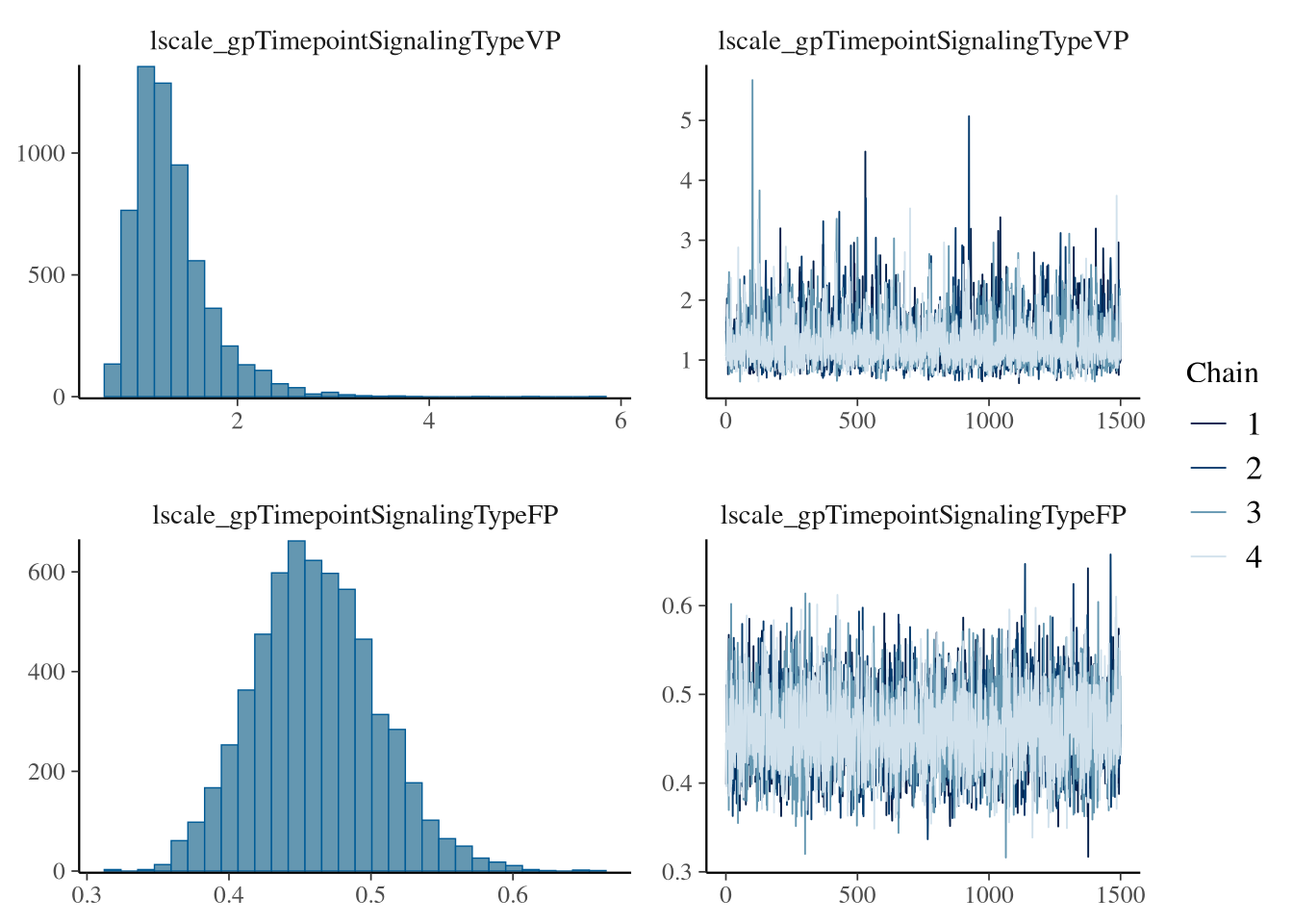
)plot(conditional_effects(m.events.f.InDegree.fit_prior, ndraws = 20, spaghetti = TRUE), points = F, ask = F)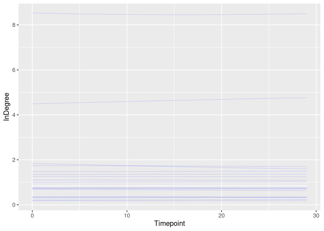
##  Family: poisson
##   Links: mu = log
## Formula: InDegree ~ gp(Timepoint, by = SignalingType)
##    Data: m.events.f.InDegree.data (Number of observations: 12840)
##   Draws: 4 chains, each with iter = 2000; warmup = 1000; thin = 1;
##          total post-warmup draws = 4000
##
## Gaussian Process Hyperparameters:
##                                    Estimate Est.Error l-95% CI u-95% CI Rhat Bulk_ESS Tail_ESS
## sdgp(gpTimepointSignalingTypeNP)       0.08      0.06     0.00     0.23 1.00     3540     1828
## sdgp(gpTimepointSignalingTypeVP)       0.08      0.06     0.00     0.22 1.00     3364     1697
## sdgp(gpTimepointSignalingTypeFP)       0.08      0.06     0.00     0.22 1.00     3095     1507
## lscale(gpTimepointSignalingTypeNP)     2.21      0.78     1.18     4.08 1.00     7405     2754
## lscale(gpTimepointSignalingTypeVP)     2.21      0.76     1.17     4.07 1.00     6215     2912
## lscale(gpTimepointSignalingTypeFP)     2.23      0.78     1.19     4.22 1.00     6676     2511
##
## Regression Coefficients:
##           Estimate Est.Error l-95% CI u-95% CI Rhat Bulk_ESS Tail_ESS
## Intercept    -0.00      1.03    -1.99     1.97 1.00     7638     2844
##
## Draws were sampled using sample(hmc). For each parameter, Bulk_ESS
## and Tail_ESS are effective sample size measures, and Rhat is the potential
## scale reduction factor on split chains (at convergence, Rhat = 1).
Model fitting
m.events.f.InDegree.fit <- brm(
  formula = m.events.f.InDegree.formula,
  prior   = m.events.f.InDegree.priors,
  data    = m.events.f.InDegree.data,
  chains = 4,
  cores = 4,
  seed = 42,
  warmup = 500,
  iter = 2000,
  file = paste0(fits_path, 'resource_discoveries_fast_in_degree.rds'),
  backend = "cmdstanr",
  threads = threading(100),
  control = list(adapt_delta = 0.95),
  save_pars = save_pars(all = TRUE)
)## Family: poisson
## Links: mu = log
## Formula: InDegree ~ gp(Timepoint, by = SignalingType)
## Data: m.events.f.InDegree.data (Number of observations: 12840)
## Draws: 4 chains, each with iter = 2000; warmup = 500; thin = 1;
## total post-warmup draws = 6000
##
## Gaussian Process Hyperparameters:
## Estimate Est.Error l-95% CI u-95% CI Rhat Bulk_ESS Tail_ESS
## sdgp(gpTimepointSignalingTypeNP) 0.09 0.06 0.01 0.23 1.00 2529 2808
## sdgp(gpTimepointSignalingTypeVP) 0.20 0.06 0.10 0.33 1.00 5832 4260
## sdgp(gpTimepointSignalingTypeFP) 0.38 0.06 0.27 0.51 1.00 6580 4532
## lscale(gpTimepointSignalingTypeNP) 2.06 0.73 1.07 3.83 1.00 8533 4284
## lscale(gpTimepointSignalingTypeVP) 1.32 0.40 0.79 2.34 1.00 6536 3817
## lscale(gpTimepointSignalingTypeFP) 0.46 0.04 0.38 0.55 1.00 7060 4615
##
## Regression Coefficients:
## Estimate Est.Error l-95% CI u-95% CI Rhat Bulk_ESS Tail_ESS
## Intercept 0.16 0.08 -0.04 0.31 1.00 1982 2219
##
## Draws were sampled using sample(hmc). For each parameter, Bulk_ESS
## and Tail_ESS are effective sample size measures, and Rhat is the potential
## scale reduction factor on split chains (at convergence, Rhat = 1).Model diagnostics
m.events.f.InDegree.me <- conditional_effects(m.events.f.InDegree.fit, ndraws = 200, spaghetti = TRUE)
plot(m.events.f.InDegree.me, ask = FALSE, points = F)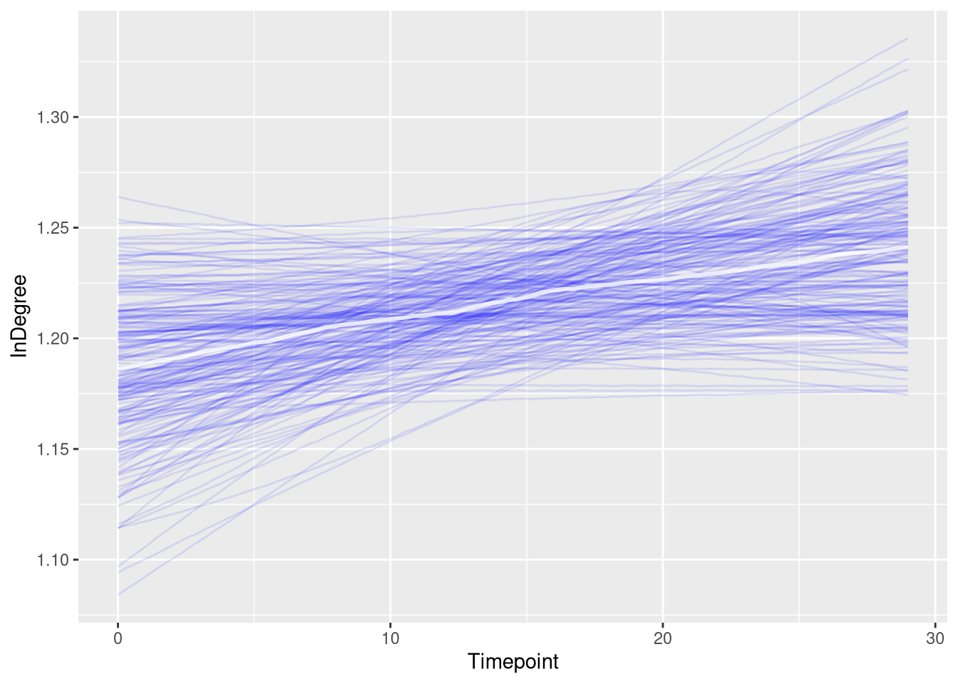
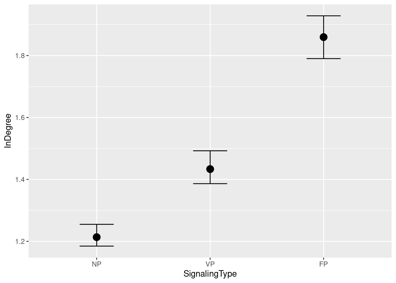
Statistical Comparisons
m.events.f.InDegree.fit %>%
  emmeans(~ SignalingType,
          at = list(Timepoint = 10),
          epred = TRUE,
          type = "response") %>%
  contrast(method = "revpairwise", simple = "each", combine = TRUE) %>%
  gather_emmeans_draws() %>%
  mean_hdci(.width = 0.9) %>%
  mutate(.value = round(.value, 2), .lower = round(.lower, 2), .upper = round(.upper, 2)) %>%
  kable("html", digits = 2) %>%
kable_classic(full_width = T, position = "center")| contrast | .value | .lower | .upper | .width | .point | .interval |
|---|---|---|---|---|---|---|
| FP - NP | 0.80 | 0.72 | 0.88 | 0.9 | mean | hdci |
| FP - VP | 0.62 | 0.54 | 0.70 | 0.9 | mean | hdci |
| VP - NP | 0.18 | 0.13 | 0.23 | 0.9 | mean | hdci |
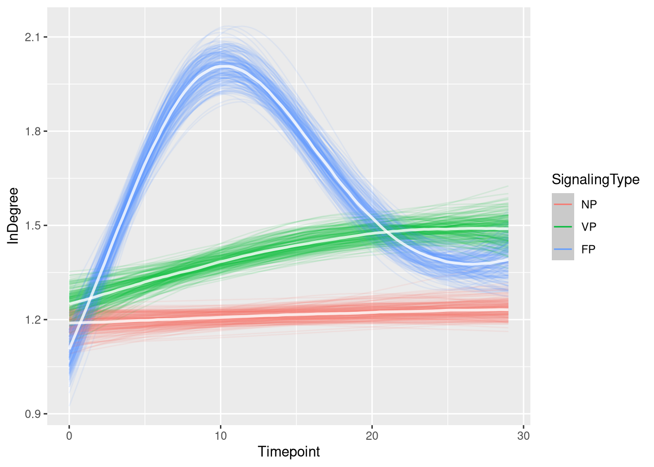
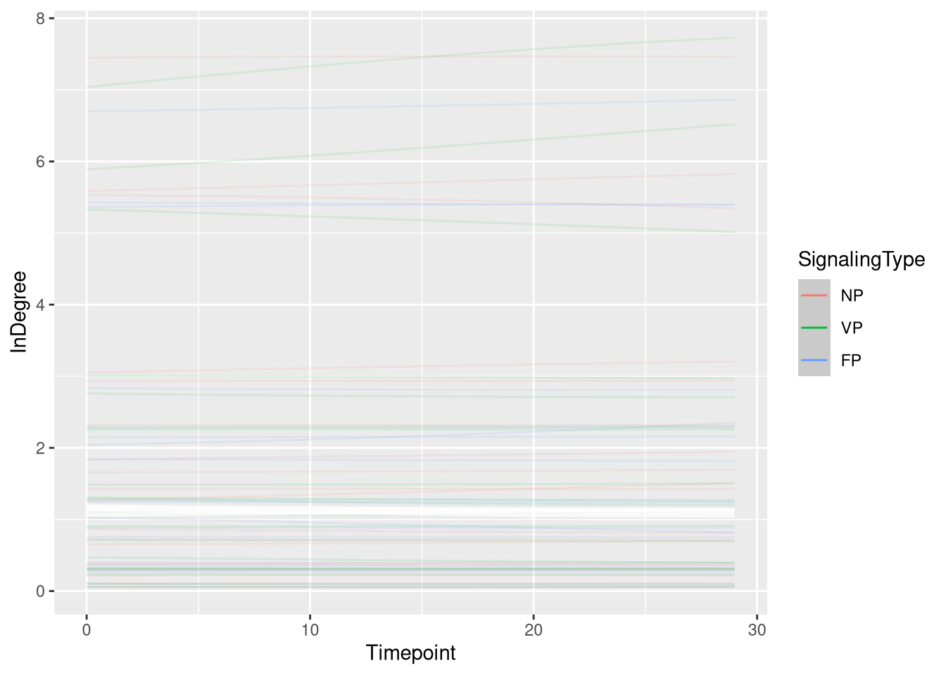
Figure
m.events.f.InDegree.draws <- m.events.f.InDegree.data %>%
  mutate(SignalingType = factor(SignalingType, levels = c('NP', 'VP', 'FP'))) %>%
  data_grid(Timepoint, SignalingType) %>%
  tidybayes::add_epred_draws(m.events.f.InDegree.fit, allow_new_levels = TRUE, re_formula = m.events.f.InDegree.formula)
events_fast_in_degree_fig <- m.events.f.InDegree.draws %>%
ggplot(aes(x = Timepoint, y = .epred, fill = SignalingType, color = SignalingType)) + # , group = SignalingType
stat_lineribbon(aes(group = paste(group, ...width..)), .width = c(.9), alpha = 1/2) +
scale_color_manual(breaks = c('NP', 'VP', 'FP'),
aesthetics = c("colour", "fill"),
values = c("#DF536B", "#61D04F", "#2297E6"),
guide = guide_legend(
title = "Signaling",
)
) +
# theme_nice(legend.pos = 'top') +
theme_clean() +
panel_border() +
theme(legend.position = "none") +
scale_x_continuous(
limits = c(0, 30),
expand = expansion(mult = c(0, 0))
) +
labs(x = "Time [s]",
y = "In Degree")
events_fast_in_degree_fig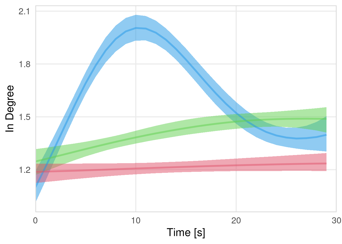
In degree (Others)
m.events.f.InDegree.Others.data <- resource_discoveries_data %>%
  filter(ResourceSpeed == 'fast', SignalingType != 'A', PlayerOrderCat == 'others') %>%
  filter(((Timepoint * 10) %% 10 == 0))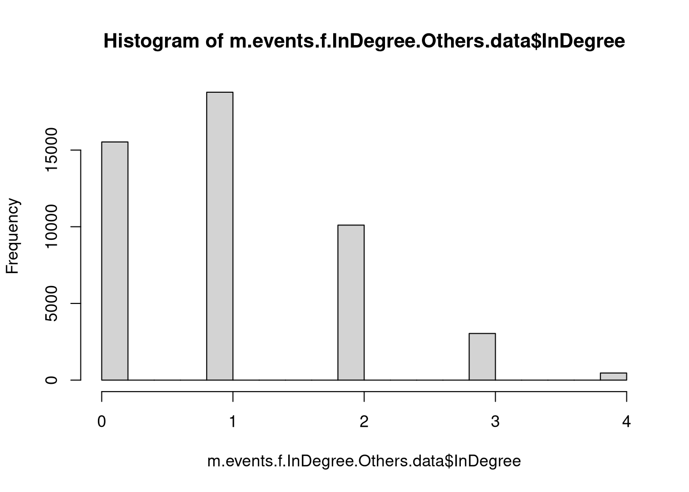
m.events.f.InDegree.Others.formula <- brmsformula(
  InDegree ~ gp(Timepoint, by = SignalingType),
  family = poisson(link = "log")
  )
m.events.f.InDegree.Others.priors <-
prior(normal(0, 1), class = "Intercept") +
prior(inv_gamma(10, 20), class = "lscale", coef = "gpTimepointSignalingTypeFP") +
prior(inv_gamma(10, 20), class = "lscale", coef = "gpTimepointSignalingTypeNP") +
prior(inv_gamma(10, 20), class = "lscale", coef = "gpTimepointSignalingTypeVP") +
prior(normal(0, 0.1), class = "sdgp", lb = 0)Prior predictive checks
m.events.f.InDegree.Others.fit_prior <- brm(
  formula = m.events.f.InDegree.Others.formula,
  prior   = m.events.f.InDegree.Others.priors,
  data    = m.events.f.InDegree.Others.data,
  chains  = 4,
  cores   = 4,
  seed    = 42,
  iter    = 2000,
  file = paste0(fits_path, 'resource_discoveries_fast_in_degree_others_prior.rds'),
  backend = "cmdstanr",
  threads = threading(100),
  control = list(adapt_delta = 0.95),
  save_pars = save_pars(all = TRUE),
  sample_prior = "only"
)plot(conditional_effects(m.events.f.InDegree.Others.fit_prior, ndraws = 20, spaghetti = TRUE), points = F, ask = F)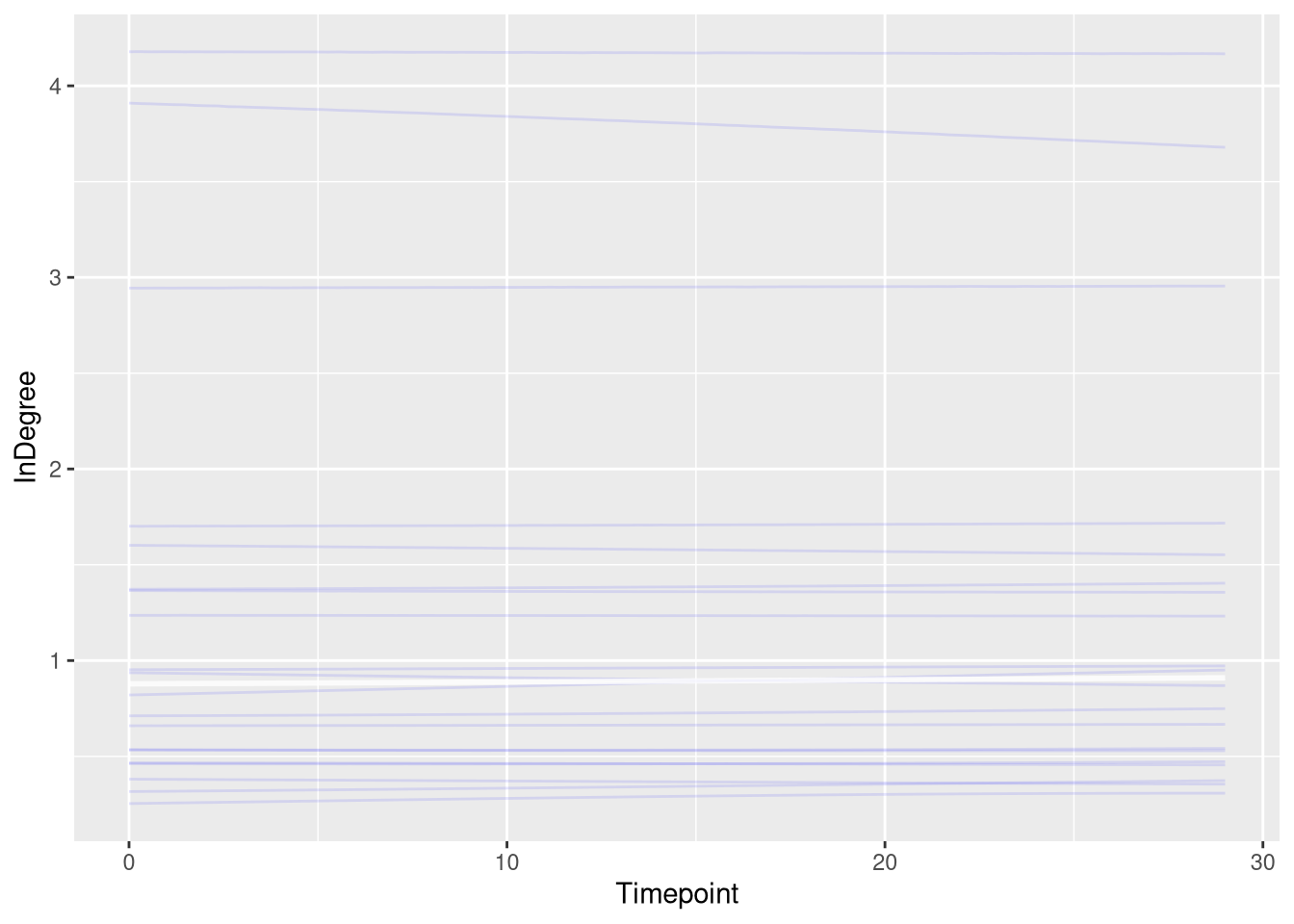
##  Family: poisson
##   Links: mu = log
## Formula: InDegree ~ gp(Timepoint, by = SignalingType)
##    Data: m.events.f.InDegree.Others.data (Number of observations: 47910)
##   Draws: 4 chains, each with iter = 2000; warmup = 1000; thin = 1;
##          total post-warmup draws = 4000
##
## Gaussian Process Hyperparameters:
##                                    Estimate Est.Error l-95% CI u-95% CI Rhat Bulk_ESS Tail_ESS
## sdgp(gpTimepointSignalingTypeNP)       0.08      0.06     0.00     0.23 1.00     3540     1828
## sdgp(gpTimepointSignalingTypeVP)       0.08      0.06     0.00     0.22 1.00     3364     1697
## sdgp(gpTimepointSignalingTypeFP)       0.08      0.06     0.00     0.22 1.00     3095     1507
## lscale(gpTimepointSignalingTypeNP)     2.21      0.78     1.18     4.08 1.00     7405     2754
## lscale(gpTimepointSignalingTypeVP)     2.21      0.76     1.17     4.07 1.00     6215     2912
## lscale(gpTimepointSignalingTypeFP)     2.23      0.78     1.19     4.22 1.00     6676     2511
##
## Regression Coefficients:
##           Estimate Est.Error l-95% CI u-95% CI Rhat Bulk_ESS Tail_ESS
## Intercept    -0.00      1.03    -1.99     1.97 1.00     7638     2844
##
## Draws were sampled using sample(hmc). For each parameter, Bulk_ESS
## and Tail_ESS are effective sample size measures, and Rhat is the potential
## scale reduction factor on split chains (at convergence, Rhat = 1).
Model fitting
m.events.f.InDegree.Others.fit <- brm(
  formula = m.events.f.InDegree.Others.formula,
  prior   = m.events.f.InDegree.Others.priors,
  data    = m.events.f.InDegree.Others.data,
  chains = 4,
  cores = 4,
  seed = 42,
  warmup = 500,
  iter = 2000,
  file = paste0(fits_path, 'resource_discoveries_fast_in_degree_others.rds'),
  backend = "cmdstanr",
  threads = threading(100),
  control = list(adapt_delta = 0.95),
  save_pars = save_pars(all = TRUE)
)## Family: poisson
## Links: mu = log
## Formula: InDegree ~ gp(Timepoint, by = SignalingType)
## Data: m.events.f.InDegree.Others.data (Number of observations: 47910)
## Draws: 4 chains, each with iter = 2000; warmup = 500; thin = 1;
## total post-warmup draws = 6000
##
## Gaussian Process Hyperparameters:
## Estimate Est.Error l-95% CI u-95% CI Rhat Bulk_ESS Tail_ESS
## sdgp(gpTimepointSignalingTypeNP) 0.16 0.06 0.07 0.29 1.00 2952 2456
## sdgp(gpTimepointSignalingTypeVP) 0.20 0.06 0.11 0.32 1.00 3501 3071
## sdgp(gpTimepointSignalingTypeFP) 0.26 0.06 0.16 0.38 1.00 3478 3626
## lscale(gpTimepointSignalingTypeNP) 1.58 0.51 0.90 2.88 1.00 4715 4145
## lscale(gpTimepointSignalingTypeVP) 1.37 0.34 0.88 2.20 1.00 5917 3981
## lscale(gpTimepointSignalingTypeFP) 0.85 0.12 0.64 1.12 1.00 3639 4049
##
## Regression Coefficients:
## Estimate Est.Error l-95% CI u-95% CI Rhat Bulk_ESS Tail_ESS
## Intercept -0.13 0.11 -0.35 0.06 1.00 1341 2472
##
## Draws were sampled using sample(hmc). For each parameter, Bulk_ESS
## and Tail_ESS are effective sample size measures, and Rhat is the potential
## scale reduction factor on split chains (at convergence, Rhat = 1).Model diagnostics
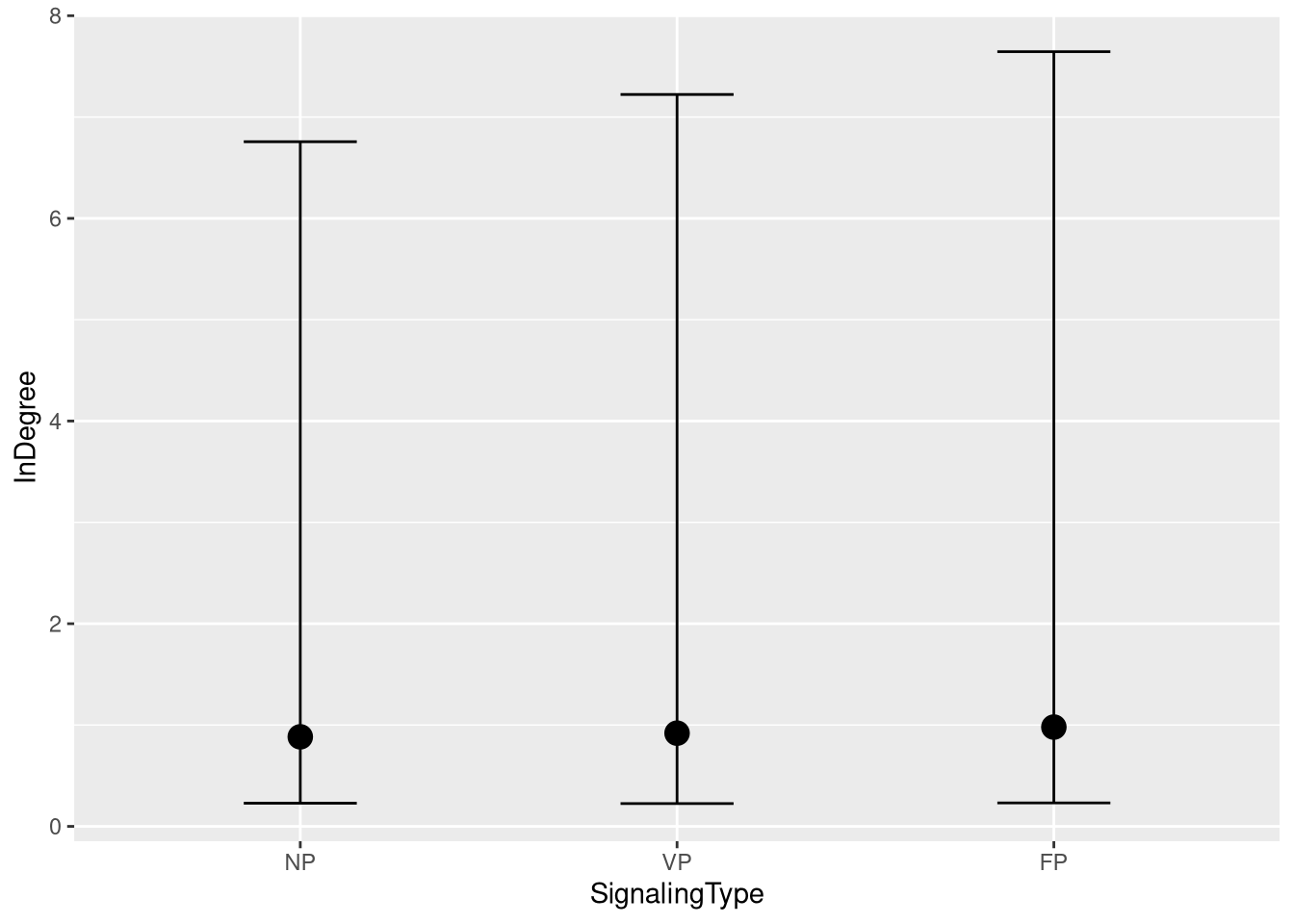
m.events.f.InDegree.Others.me <- conditional_effects(m.events.f.InDegree.Others.fit, ndraws = 200, spaghetti = TRUE)
plot(m.events.f.InDegree.Others.me, ask = FALSE, points = F)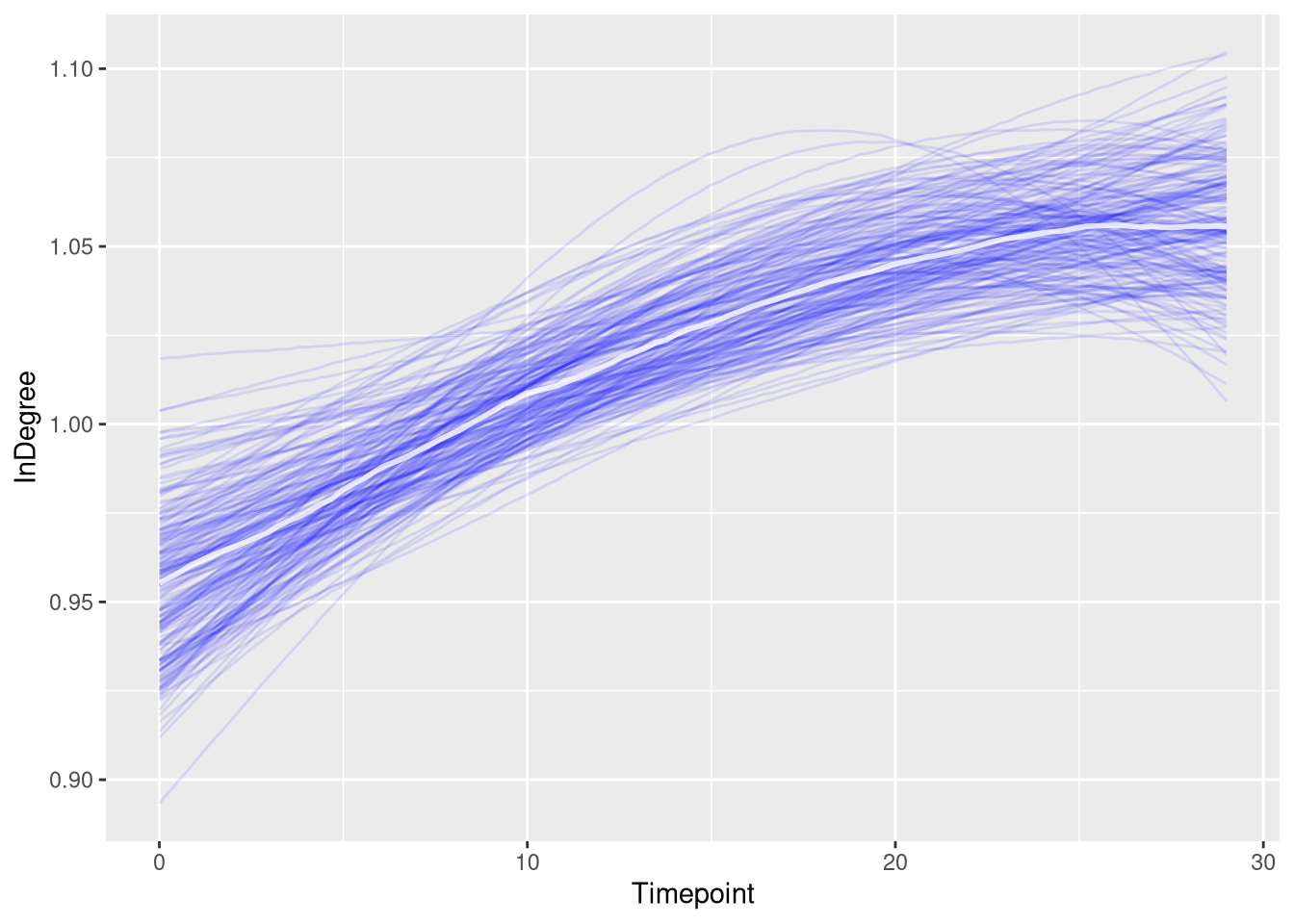
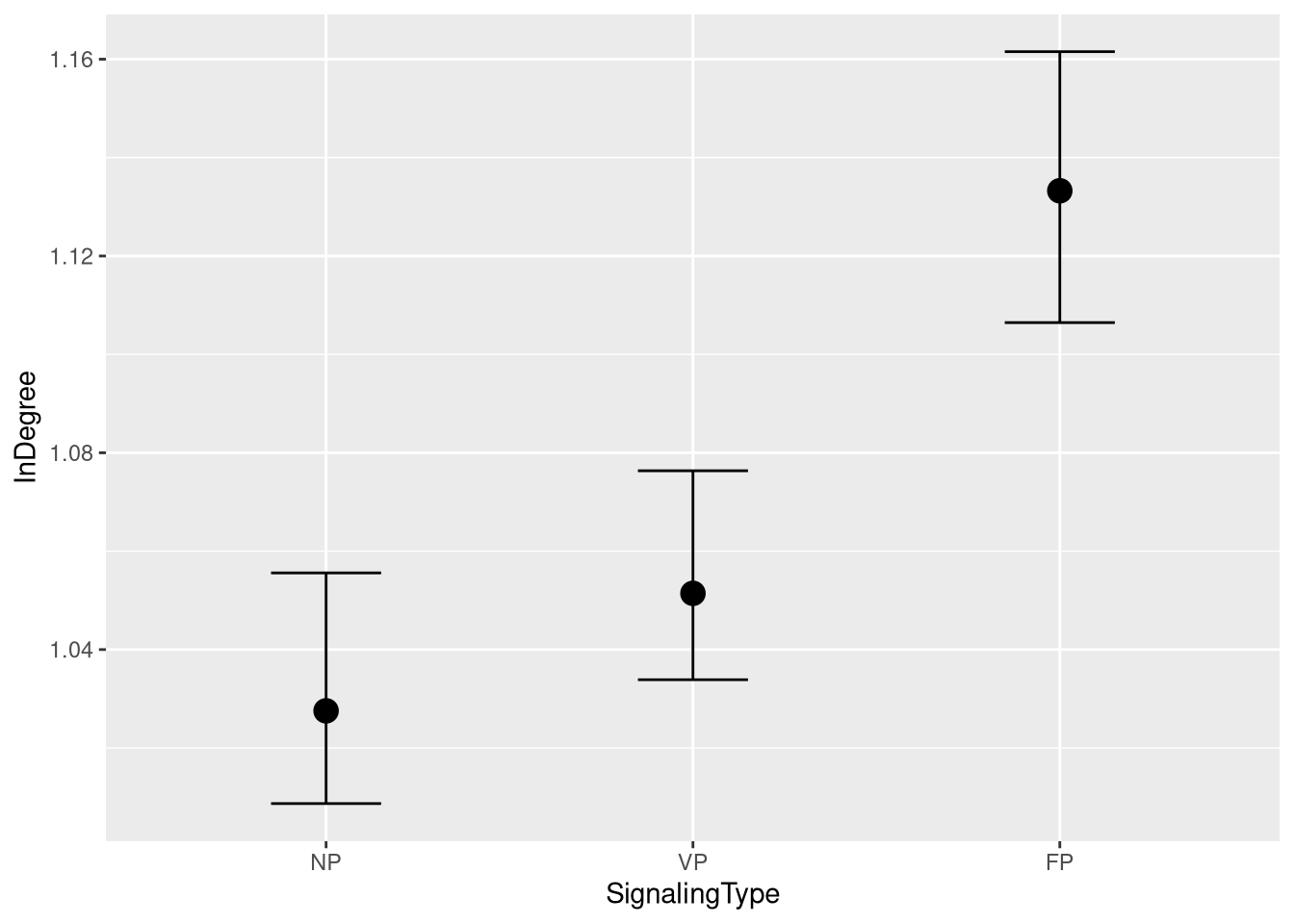
Statistical Comparisons
m.events.f.InDegree.Others.fit %>%
  emmeans(~ SignalingType,
          at = list(Timepoint = 10),
          epred = TRUE,
          type = "response") %>%
  contrast(method = "revpairwise", simple = "each", combine = TRUE) %>%
  gather_emmeans_draws() %>%
  mean_hdci(.width = 0.9) %>%
  mutate(.value = round(.value, 2), .lower = round(.lower, 2), .upper = round(.upper, 2)) %>%
  kable("html", digits = 2) %>%
kable_classic(full_width = T, position = "center")| contrast | .value | .lower | .upper | .width | .point | .interval |
|---|---|---|---|---|---|---|
| FP - NP | 0.06 | 0.03 | 0.08 | 0.9 | mean | hdci |
| FP - VP | 0.05 | 0.02 | 0.07 | 0.9 | mean | hdci |
| VP - NP | 0.01 | -0.02 | 0.03 | 0.9 | mean | hdci |
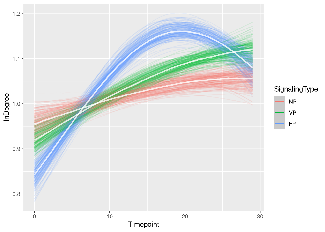
Figure
m.events.f.InDegree.Others.draws <- m.events.f.InDegree.Others.data %>%
  mutate(SignalingType = factor(SignalingType, levels = c('NP', 'VP', 'FP'))) %>%
  data_grid(Timepoint, SignalingType) %>%
  tidybayes::add_epred_draws(m.events.f.InDegree.Others.fit, allow_new_levels = TRUE, re_formula = m.events.f.InDegree.Others.formula)
events_fast_in_degree_others_fig <- m.events.f.InDegree.Others.draws %>%
ggplot(aes(x = Timepoint, y = .epred, fill = SignalingType, color = SignalingType)) + # , group = SignalingType
stat_lineribbon(aes(group = paste(group, ...width..)), .width = c(.9), alpha = 1/2) +
scale_color_manual(breaks = c('NP', 'VP', 'FP'),
aesthetics = c("colour", "fill"),
values = c("#DF536B", "#61D04F", "#2297E6"),
guide = guide_legend(
title = "Signaling",
)
) +
# theme_nice(legend.pos = 'top') +
theme_clean() +
panel_border() +
theme(legend.position = "none") +
scale_x_continuous(
limits = c(0, 30),
expand = expansion(mult = c(0, 0))
) +
labs(x = "Time [s]",
y = "In Degree")
events_fast_in_degree_others_fig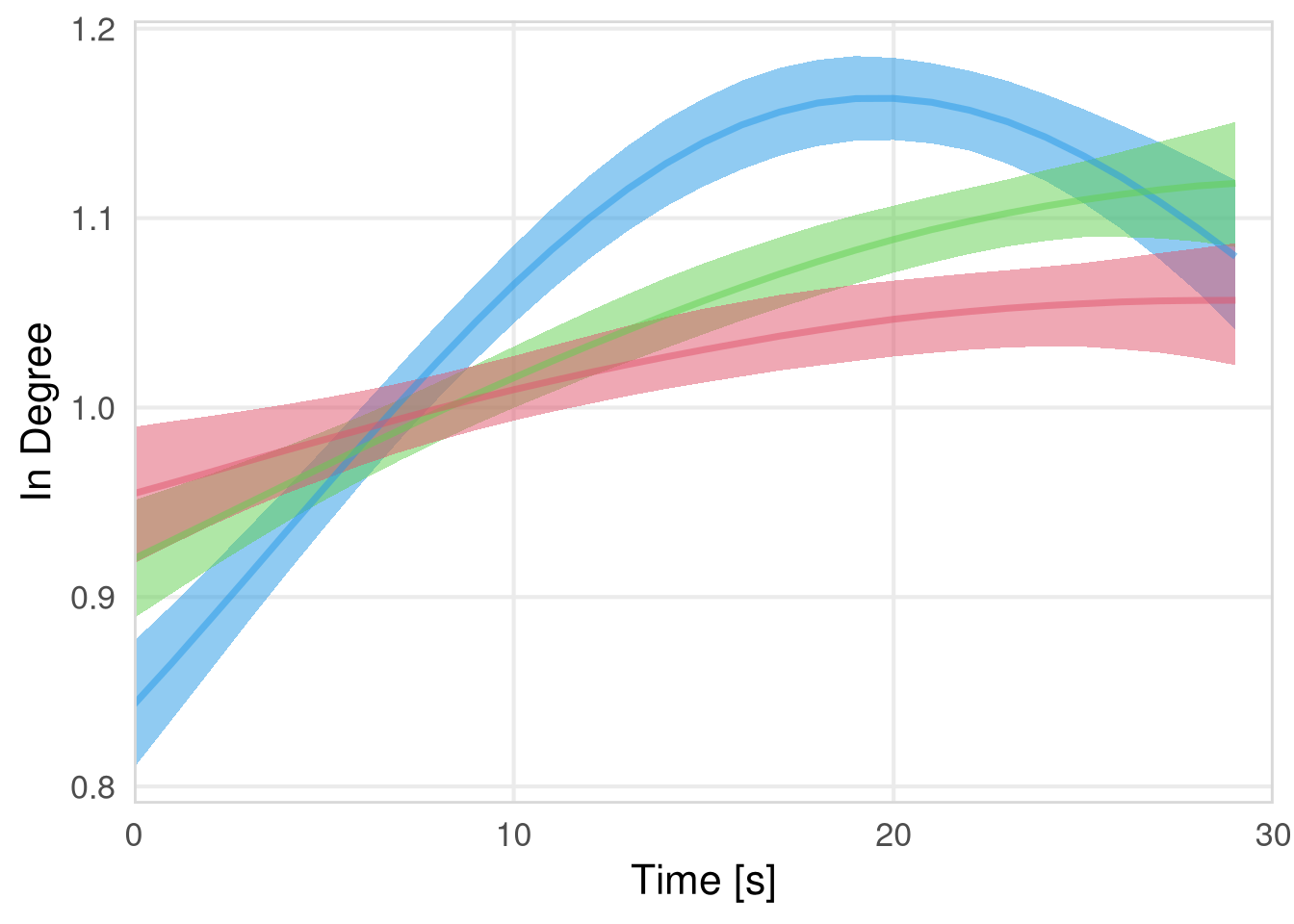
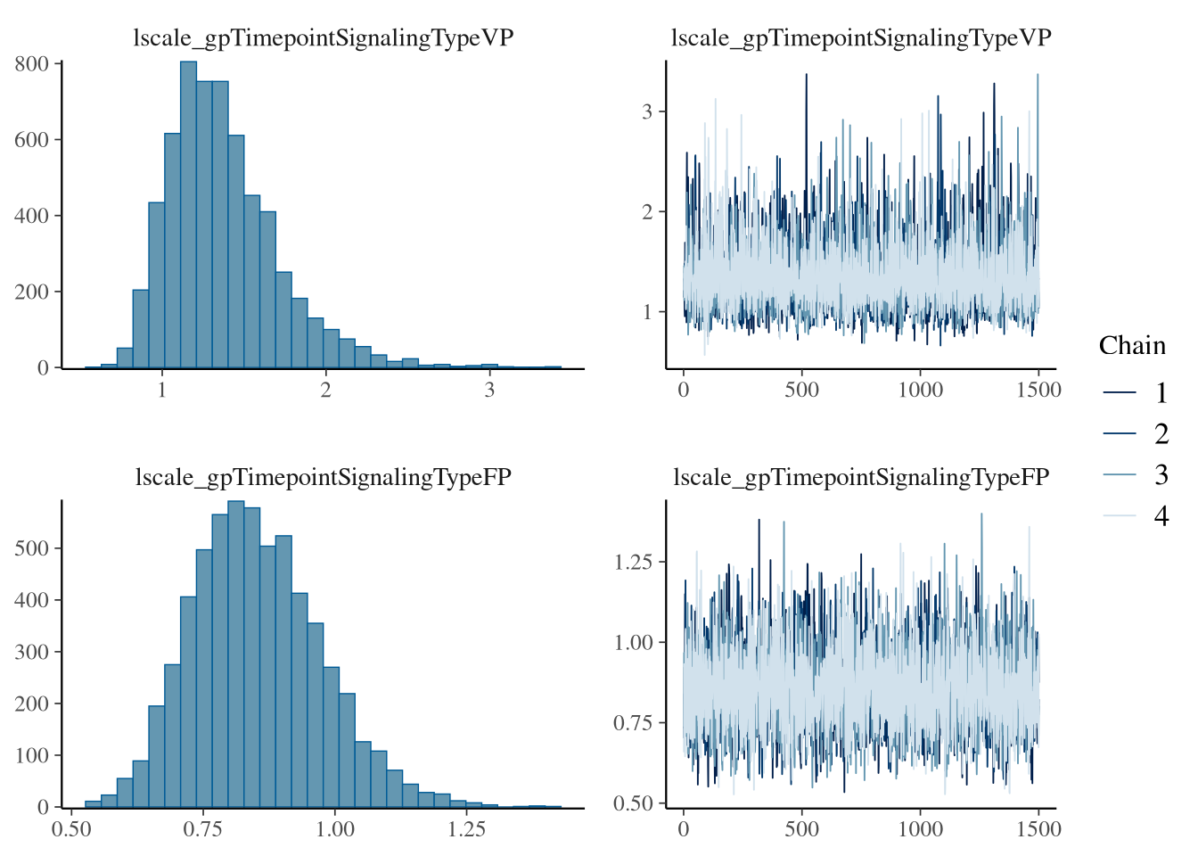
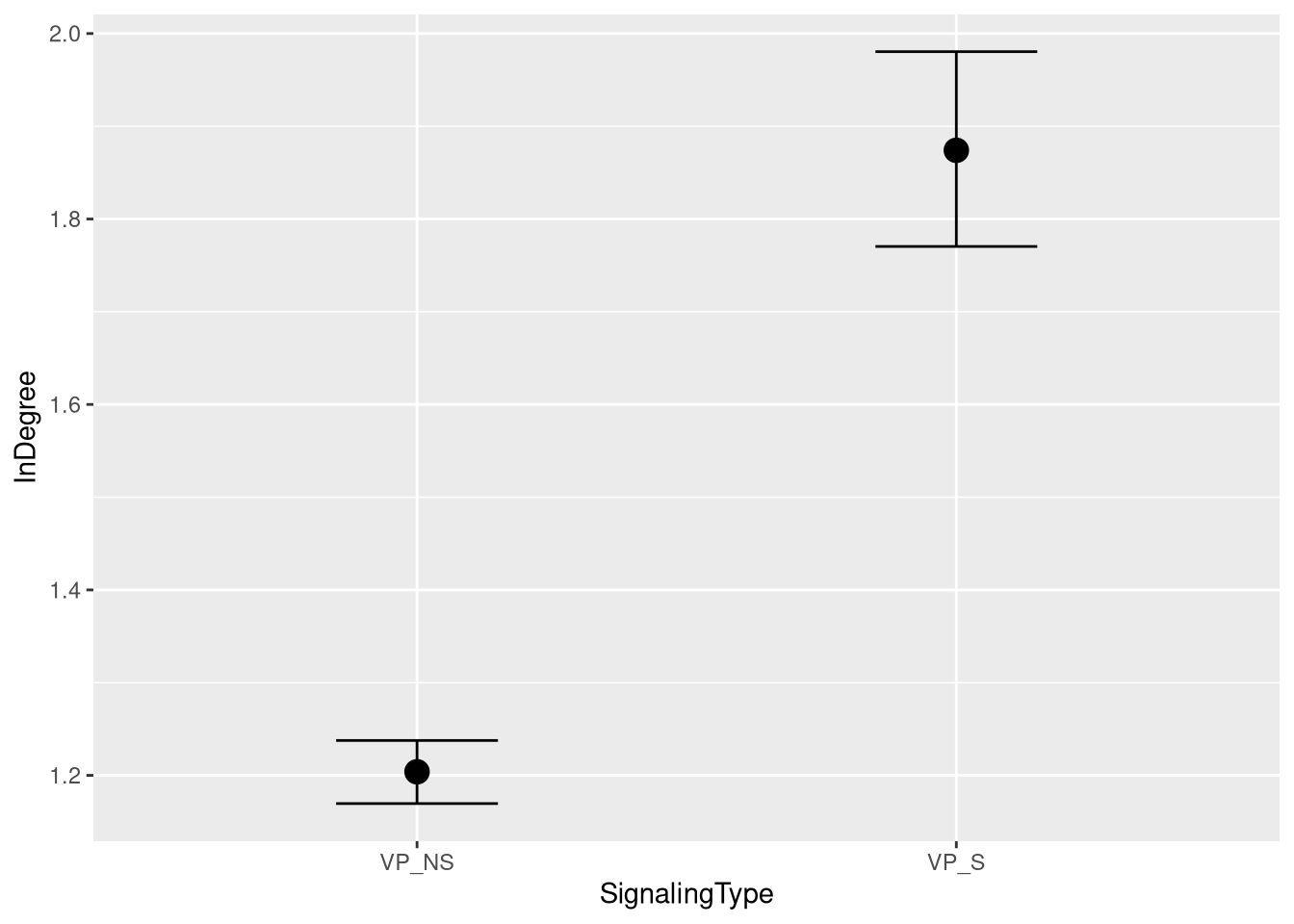
In degree VP
m.events.f.InDegree.VP.data <- resource_discoveries_data_vp %>%
  filter(ResourceSpeed == 'fast', PlayerOrderCat == 'first') %>%
  filter(((Timepoint * 10) %% 10 == 0))
m.events.f.InDegree.VP.formula <- brmsformula(
  InDegree ~ gp(Timepoint, by = SignalingType),
  family = negbinomial()
  )
m.events.f.InDegree.VP.priors <-
prior(normal(0, 1), class = "Intercept") +
prior(inv_gamma(10, 20), class = "lscale", coef = "gpTimepointSignalingTypeVP_NS") +
prior(inv_gamma(10, 20), class = "lscale", coef = "gpTimepointSignalingTypeVP_S") +
prior(normal(0, 0.1), class = "sdgp", lb = 0)Prior predictive checks
m.events.f.InDegree.VP.fit_prior <- brm(
  formula = m.events.f.InDegree.VP.formula,
  prior   = m.events.f.InDegree.VP.priors,
  data    = m.events.f.InDegree.VP.data,
  chains  = 4,
  cores   = 4,
  seed    = 42,
  iter    = 2000,
  file = paste0(fits_path, 'resource_discoveries_fast_in_degree_vp_prior.rds'),
  backend = "cmdstanr",
  threads = threading(100),
  control = list(adapt_delta = 0.95),
  save_pars = save_pars(all = TRUE),
  sample_prior = "only"
)plot(conditional_effects(m.events.f.InDegree.VP.fit_prior, ndraws = 20, spaghetti = TRUE), points = F, ask = F)
##  Family: negbinomial
##   Links: mu = log; shape = identity
## Formula: InDegree ~ gp(Timepoint, by = SignalingType)
##    Data: m.events.f.InDegree.VP.data (Number of observations: 5010)
##   Draws: 4 chains, each with iter = 2000; warmup = 1000; thin = 1;
##          total post-warmup draws = 4000
##
## Gaussian Process Hyperparameters:
##                                       Estimate Est.Error l-95% CI u-95% CI Rhat Bulk_ESS Tail_ESS
## sdgp(gpTimepointSignalingTypeVP_NS)       0.08      0.06     0.00     0.22 1.00     3635     1707
## sdgp(gpTimepointSignalingTypeVP_S)        0.08      0.06     0.00     0.22 1.00     3614     1899
## lscale(gpTimepointSignalingTypeVP_NS)     2.23      0.80     1.14     4.27 1.00     5093     2773
## lscale(gpTimepointSignalingTypeVP_S)      2.24      0.82     1.15     4.34 1.00     5575     2501
##
## Regression Coefficients:
##           Estimate Est.Error l-95% CI u-95% CI Rhat Bulk_ESS Tail_ESS
## Intercept     0.01      0.99    -1.93     1.91 1.00     5944     2882
##
## Further Distributional Parameters:
##         Estimate    Est.Error l-95% CI u-95% CI Rhat Bulk_ESS Tail_ESS
## shape 3114684.60 195245161.46     0.13  4205.25 1.00     3644     1972
##
## Draws were sampled using sample(hmc). For each parameter, Bulk_ESS
## and Tail_ESS are effective sample size measures, and Rhat is the potential
## scale reduction factor on split chains (at convergence, Rhat = 1).
Model fitting
m.events.f.InDegree.VP.fit <- brm(
  formula = m.events.f.InDegree.VP.formula,
  prior   = m.events.f.InDegree.VP.priors,
  data    = m.events.f.InDegree.VP.data,
  chains = 4,
  cores = 4,
  seed = 42,
  warmup = 500,
  iter = 2000,
  file = paste0(fits_path, 'resource_discoveries_fast_in_degree_vp.rds'),
  backend = "cmdstanr",
  threads = threading(100),
  control = list(adapt_delta = 0.95),
  save_pars = save_pars(all = TRUE)
)## Family: negbinomial
## Links: mu = log; shape = identity
## Formula: InDegree ~ gp(Timepoint, by = SignalingType)
## Data: m.events.f.InDegree.VP.data (Number of observations: 5010)
## Draws: 4 chains, each with iter = 2000; warmup = 500; thin = 1;
## total post-warmup draws = 6000
##
## Gaussian Process Hyperparameters:
## Estimate Est.Error l-95% CI u-95% CI Rhat Bulk_ESS Tail_ESS
## sdgp(gpTimepointSignalingTypeVP_NS) 0.07 0.05 0.00 0.20 1.00 3060 2575
## sdgp(gpTimepointSignalingTypeVP_S) 0.30 0.06 0.19 0.42 1.00 5837 4345
## lscale(gpTimepointSignalingTypeVP_NS) 2.27 0.81 1.20 4.23 1.00 9775 3902
## lscale(gpTimepointSignalingTypeVP_S) 0.80 0.12 0.60 1.05 1.00 5725 4659
##
## Regression Coefficients:
## Estimate Est.Error l-95% CI u-95% CI Rhat Bulk_ESS Tail_ESS
## Intercept 0.18 0.07 0.01 0.32 1.00 2549 1906
##
## Further Distributional Parameters:
## Estimate Est.Error l-95% CI u-95% CI Rhat Bulk_ESS Tail_ESS
## shape 84354015.81 4507522747.43 413.58 10727745.00 1.00 4772 2583
##
## Draws were sampled using sample(hmc). For each parameter, Bulk_ESS
## and Tail_ESS are effective sample size measures, and Rhat is the potential
## scale reduction factor on split chains (at convergence, Rhat = 1).Model diagnostics
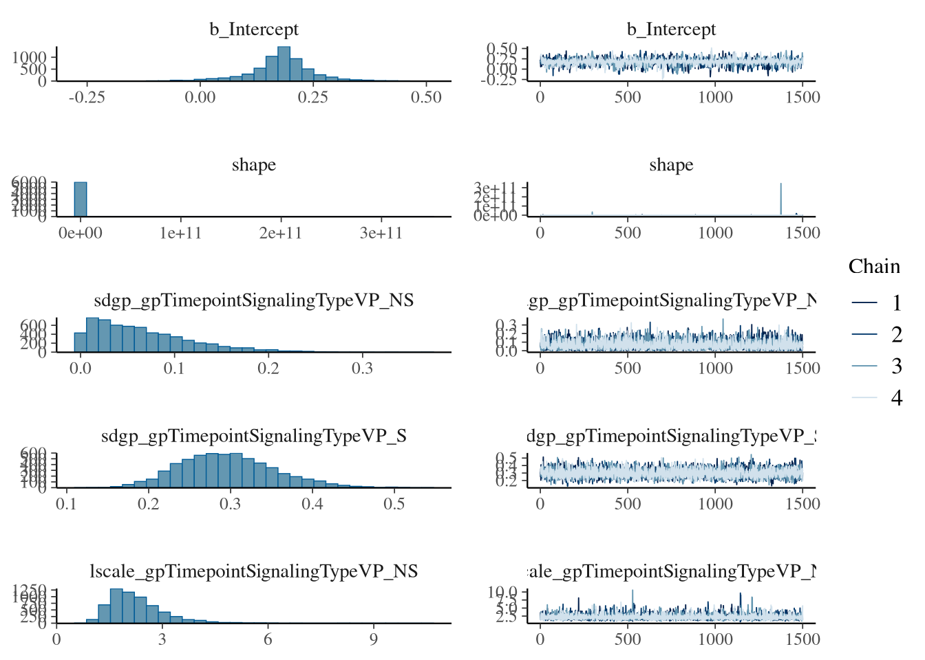
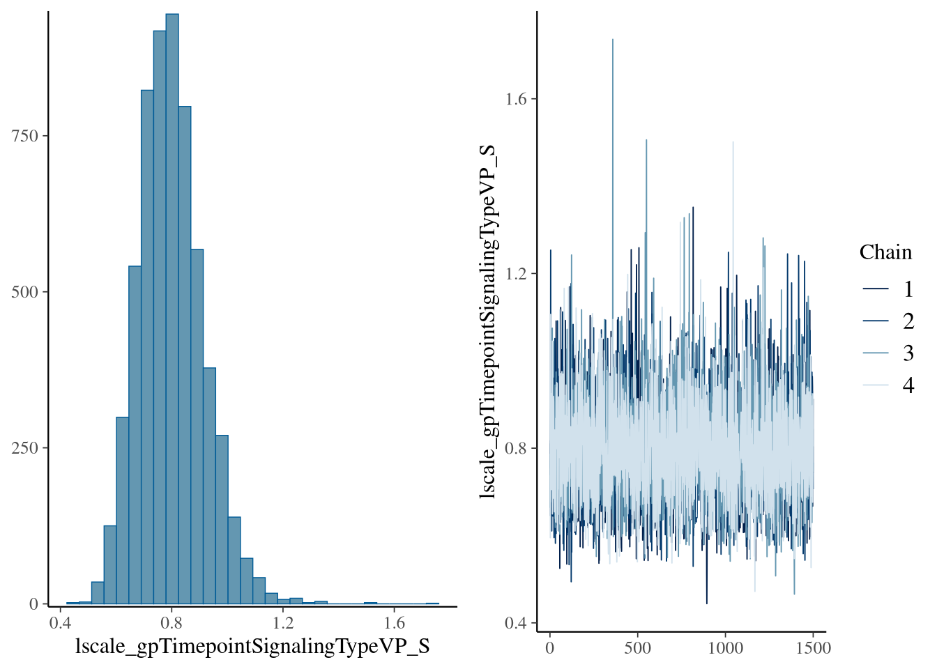
m.events.f.InDegree.VP.me <- conditional_effects(m.events.f.InDegree.VP.fit, ndraws = 200, spaghetti = TRUE)
plot(m.events.f.InDegree.VP.me, ask = FALSE, points = F)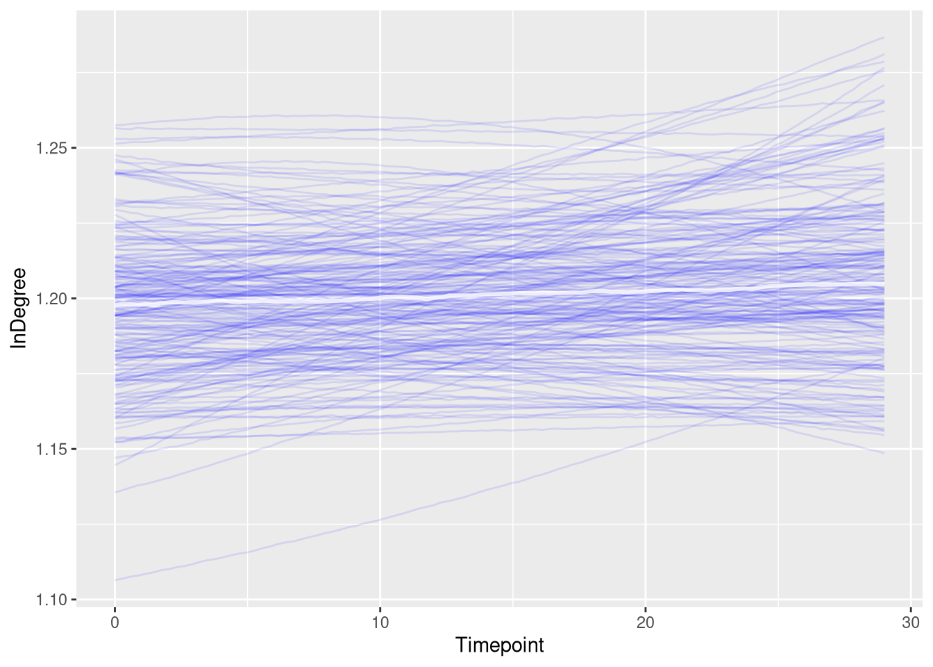
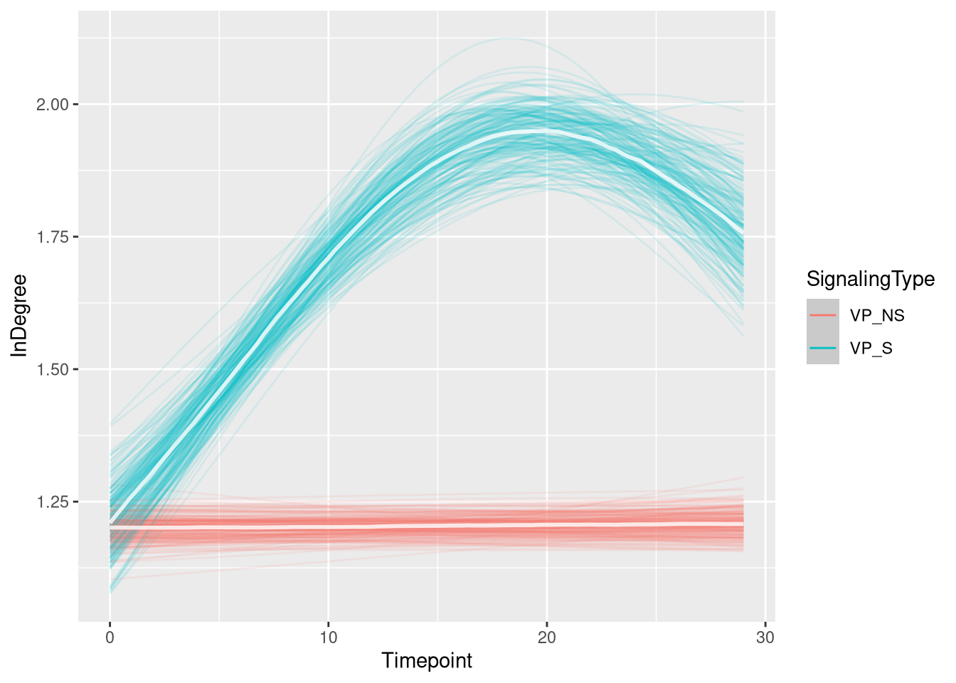
Figure
m.events.f.InDegree.VP.draws <- m.events.f.InDegree.VP.data %>%
  mutate(SignalingType = factor(SignalingType, levels = c('VP_NS', 'VP_S'))) %>%
  data_grid(Timepoint, SignalingType) %>%
  tidybayes::add_epred_draws(m.events.f.InDegree.VP.fit, allow_new_levels = TRUE, re_formula = m.events.f.InDegree.VP.formula)
events_fast_in_degree_vp_fig <- m.events.f.InDegree.VP.draws %>%
ggplot(aes(x = Timepoint, y = .epred, fill = SignalingType, color = SignalingType)) + # , group = SignalingType
stat_lineribbon(aes(group = paste(group, ...width..)), .width = c(.9), alpha = 1/2) +
theme_nice(legend.pos = 'none') +
scale_color_manual(breaks = c('VP_NS', 'VP_S'),
aesthetics = c("colour", "fill"),
values = c("#000000", "#DF536B"),
guide = guide_legend(
title = "Signaling",
)
) +
theme_clean() +
panel_border() +
theme(legend.position = "none") +
scale_x_continuous(
limits = c(0, 30),
expand = expansion(mult = c(0, 0))
) +
labs(x = "Time [s]",
y = "In Degree")
events_fast_in_degree_vp_fig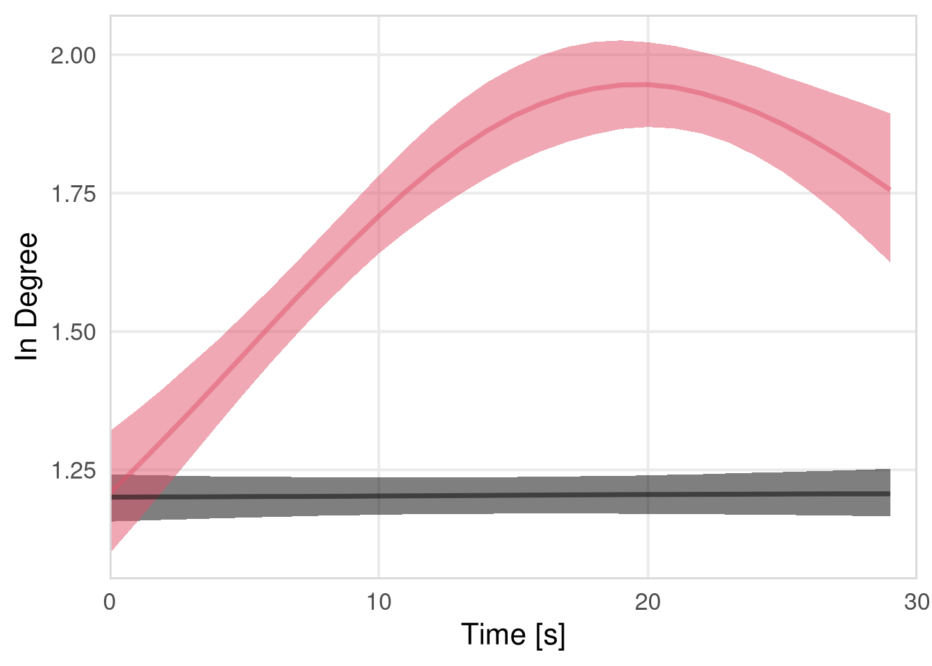
Combine plot
resource_discoveries_figure_fast <- ggarrange(
  ggarrange(events_fast_p_stay_fig,  events_fast_in_degree_fig, nrow = 2, labels = c("", "")), # c("A", "C")
  ggarrange(events_fast_p_reach_fig, events_fast_outdegree_fig, nrow = 2, labels = c("", "")), # c("B", "D")
  ncol = 2,
  widths = c(1, 1)
)

resource_discoveries_figure_fast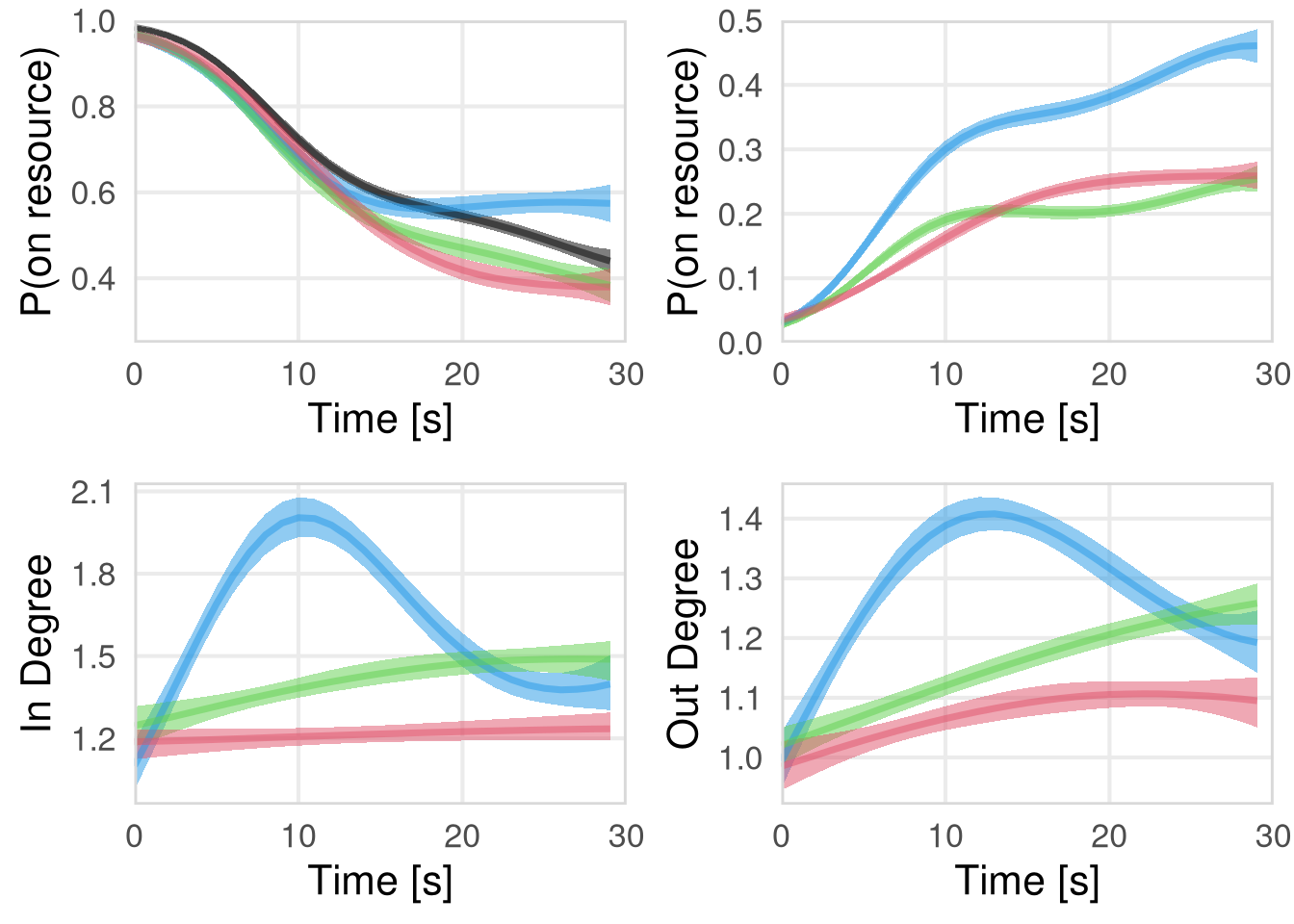
Combine plot (in/out degree full)
resource_discoveries_figure_fast_in_out_full <- ggarrange(
  ggarrange(events_fast_in_degree_fig + scale_y_continuous(limits  = c(0.75, 2.1)), #  + labs(x = "")
            events_fast_outdegree_discoverer_fig + scale_y_continuous(limits  = c(0.35, 1.45)),
            nrow = 2, labels = c("", "")),
  ggarrange(events_fast_in_degree_others_fig + scale_y_continuous(limits  = c(0.75, 2.1)), # + labs(x = "", y = "")
            events_fast_outdegree_fig + scale_y_continuous(limits  = c(0.35, 1.45)),
            nrow = 2, labels = c("", "")),
  ncol = 2,
  widths = c(1, 1)
)

resource_discoveries_figure_fast_in_out_full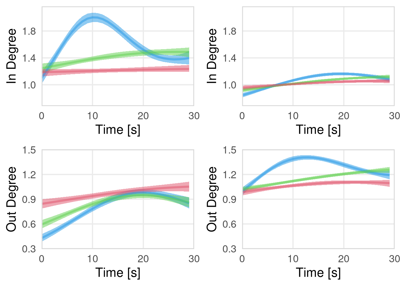
Combine plot VP
resource_discoveries_figure_fast_vp <- ggarrange(
  ggarrange(events_fast_p_stay_vp_fig,  events_fast_in_degree_vp_fig, nrow = 2, labels = c("", "")),
  ggarrange(events_fast_p_reach_vp_fig, events_fast_outdegree_vp_fig, nrow = 2, labels = c("", "")),
  ncol = 2,
  widths = c(1, 1)
)

resource_discoveries_figure_fast_vp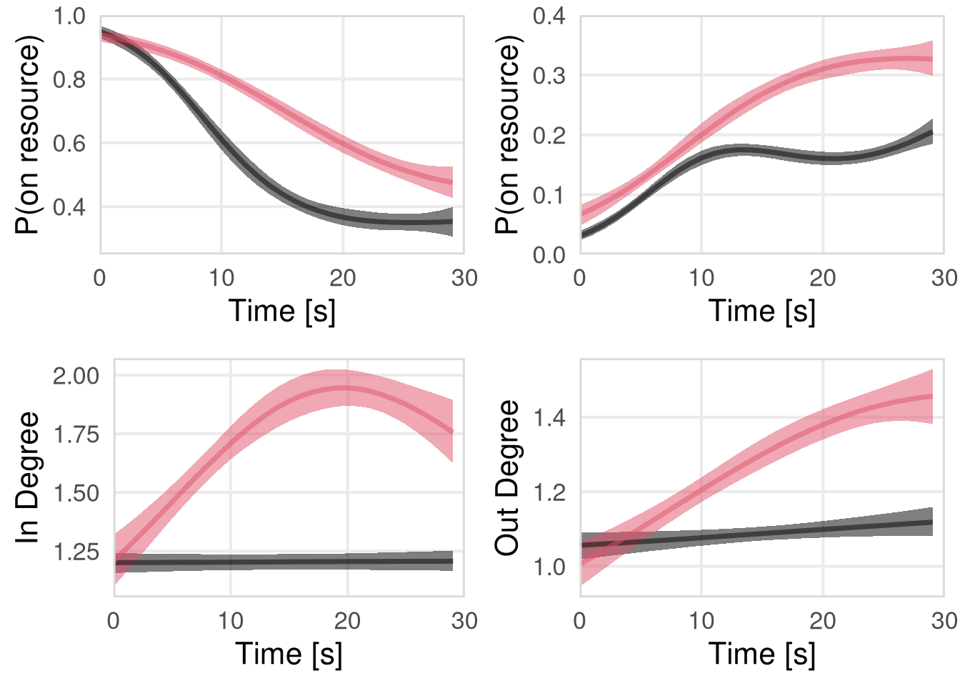
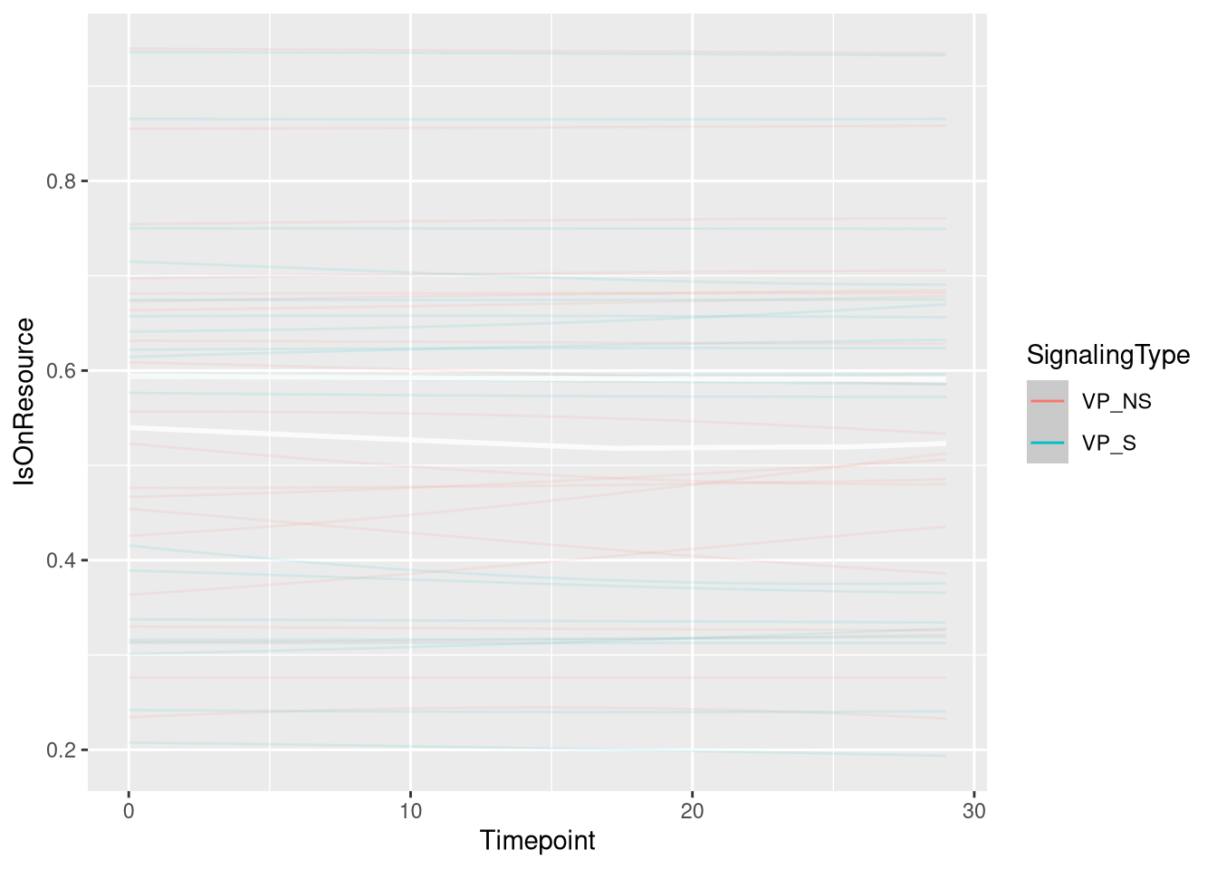
Slow
Probability of staying on resource
m.events.s.pstay.data <- resource_discoveries_data %>%
  filter(ResourceSpeed == 'slow', PlayerOrderCat == 'first') %>%
  filter(((Timepoint * 10) %% 10 == 0))


m.events.s.pstay.formula <- brmsformula(
  IsOnResource ~ gp(Timepoint, by = SignalingType),
  family = bernoulli(link = "logit")
  )
m.events.s.pstay.priors <-
prior(normal(0, 1), class = "Intercept") +
prior(inv_gamma(10, 20), class = "lscale", coef = "gpTimepointSignalingTypeA") +
prior(inv_gamma(10, 20), class = "lscale", coef = "gpTimepointSignalingTypeFP") +
prior(inv_gamma(10, 20), class = "lscale", coef = "gpTimepointSignalingTypeNP") +
prior(inv_gamma(10, 20), class = "lscale", coef = "gpTimepointSignalingTypeVP") +
prior(normal(0, 0.25), class = "sdgp", lb = 0)Prior predictive checks
m.events.s.pstay.fit_prior <- brm(
  formula = m.events.s.pstay.formula,
  prior   = m.events.s.pstay.priors,
  data    = m.events.s.pstay.data,
  chains  = 4,
  cores   = 4,
  seed    = 42,
  iter    = 2000,
  file = paste0(fits_path, 'resource_discoveries_slow_p_stay_prior.rds'),
  backend = "cmdstanr",
  threads = threading(100),
  control = list(adapt_delta = 0.95),
  save_pars = save_pars(all = TRUE),
  sample_prior = "only"
)plot(conditional_effects(m.events.f.pstay.fit_prior, ndraws = 20, spaghetti = TRUE), points = F, ask = F)
Model fitting
m.events.s.pstay.fit <- brm(
  formula = m.events.s.pstay.formula,
  prior   = m.events.s.pstay.priors,
  data    = m.events.s.pstay.data,
  chains = 4,
  cores = 4,
  seed = 42,
  warmup = 500,
  iter = 2000,
  file = paste0(fits_path, 'resource_discoveries_slow_p_stay.rds'),
  backend = "cmdstanr",
  threads = threading(100),
  control = list(adapt_delta = 0.95),
  save_pars = save_pars(all = TRUE)
)## Family: bernoulli
## Links: mu = logit
## Formula: IsOnResource ~ gp(Timepoint, by = SignalingType)
## Data: m.events.s.pstay.data (Number of observations: 7740)
## Draws: 4 chains, each with iter = 2000; warmup = 500; thin = 1;
## total post-warmup draws = 6000
##
## Gaussian Process Hyperparameters:
## Estimate Est.Error l-95% CI u-95% CI Rhat Bulk_ESS Tail_ESS
## sdgp(gpTimepointSignalingTypeA) 1.02 0.15 0.74 1.34 1.00 6695 4744
## sdgp(gpTimepointSignalingTypeNP) 0.25 0.18 0.01 0.65 1.00 2998 3009
## sdgp(gpTimepointSignalingTypeVP) 0.78 0.15 0.52 1.10 1.00 8147 4432
## sdgp(gpTimepointSignalingTypeFP) 0.58 0.18 0.21 0.93 1.00 3323 1618
## lscale(gpTimepointSignalingTypeA) 0.65 0.12 0.47 0.92 1.00 5301 4839
## lscale(gpTimepointSignalingTypeNP) 2.06 0.74 1.08 3.88 1.00 8893 4552
## lscale(gpTimepointSignalingTypeVP) 1.02 0.22 0.67 1.52 1.00 9554 5104
## lscale(gpTimepointSignalingTypeFP) 1.50 0.48 0.88 2.66 1.00 5640 4067
##
## Regression Coefficients:
## Estimate Est.Error l-95% CI u-95% CI Rhat Bulk_ESS Tail_ESS
## Intercept 1.27 0.22 0.83 1.75 1.00 3015 2781
##
## Draws were sampled using sample(hmc). For each parameter, Bulk_ESS
## and Tail_ESS are effective sample size measures, and Rhat is the potential
## scale reduction factor on split chains (at convergence, Rhat = 1).Model diagnostics
 #### Figure
m.events.s.pstay.draws <- m.events.s.pstay.data %>%
  mutate(SignalingType = factor(SignalingType, levels = c('A', 'NP', 'VP', 'FP'))) %>%
  data_grid(Timepoint, SignalingType) %>%
  tidybayes::add_epred_draws(m.events.s.pstay.fit, allow_new_levels = TRUE,
                             re_formula = m.events.s.pstay.formula)
events_slow_p_stay_fig <- m.events.s.pstay.draws %>%
ggplot(aes(x = Timepoint, y = .epred, fill = SignalingType, color = SignalingType)) +
stat_lineribbon(aes(group = paste(group, ...width..)), .width = c(.9), alpha = 1/2) +
theme_clean() +
panel_border() +
theme(legend.position = "none") +
scale_color_manual(breaks = c('A', 'NP', 'VP', 'FP'),
aesthetics = c("colour", "fill"),
values = c("#000000", "#DF536B", "#61D04F", "#2297E6"),
guide = guide_legend(
title = "Signaling",
)
) +
scale_y_continuous(
limits = c(0.4, 1.0),
expand = expansion(mult = c(0, 0))
) +
scale_x_continuous(
limits = c(0, 30),
expand = expansion(mult = c(0, 0))
) +
labs(x = "Time [s]",
y = "P(on resource)")
events_slow_p_stay_fig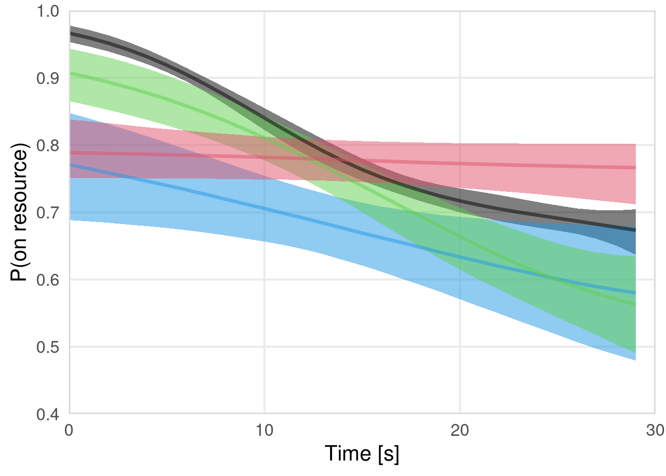
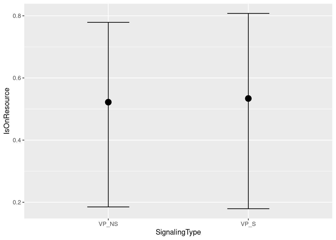
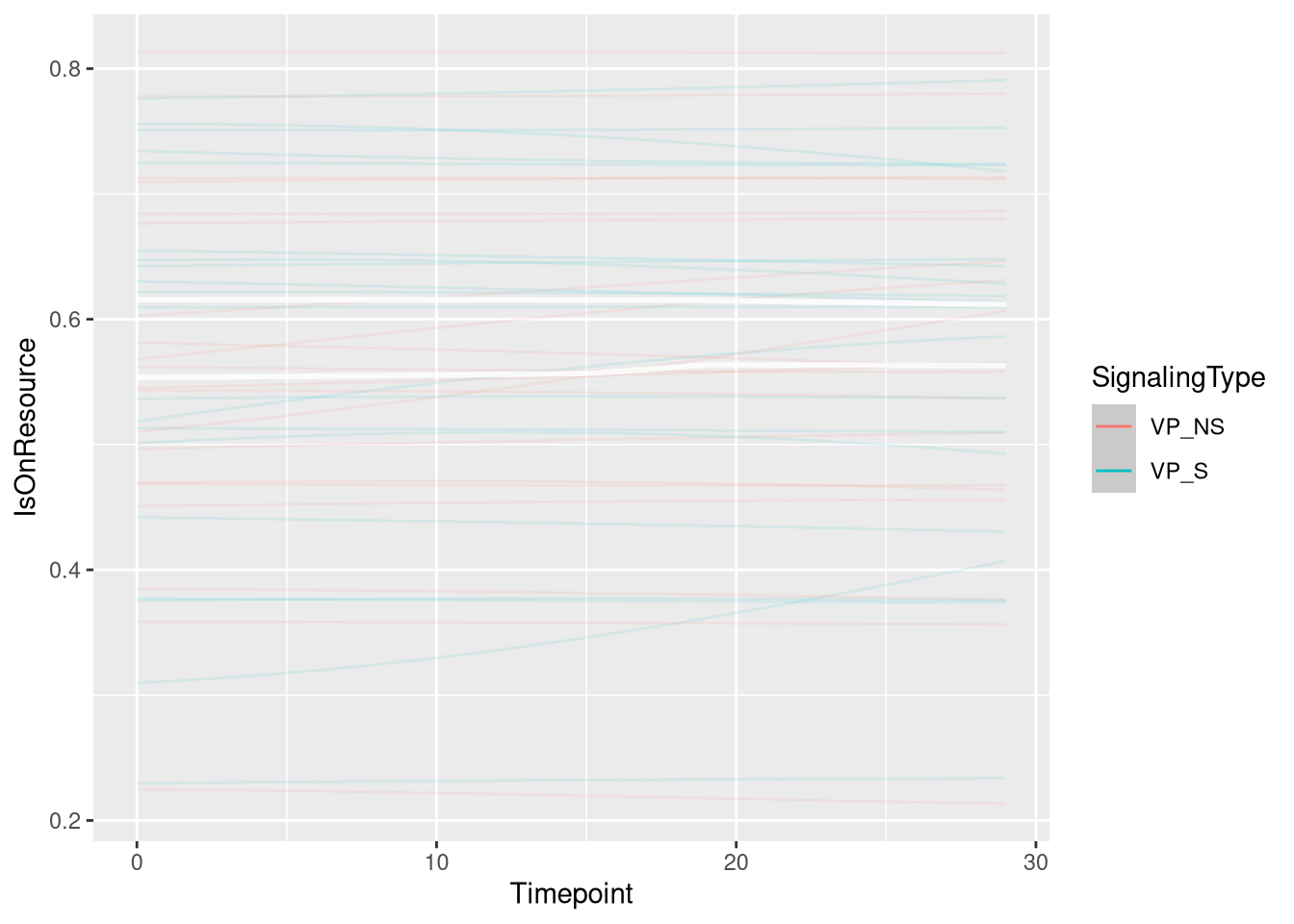
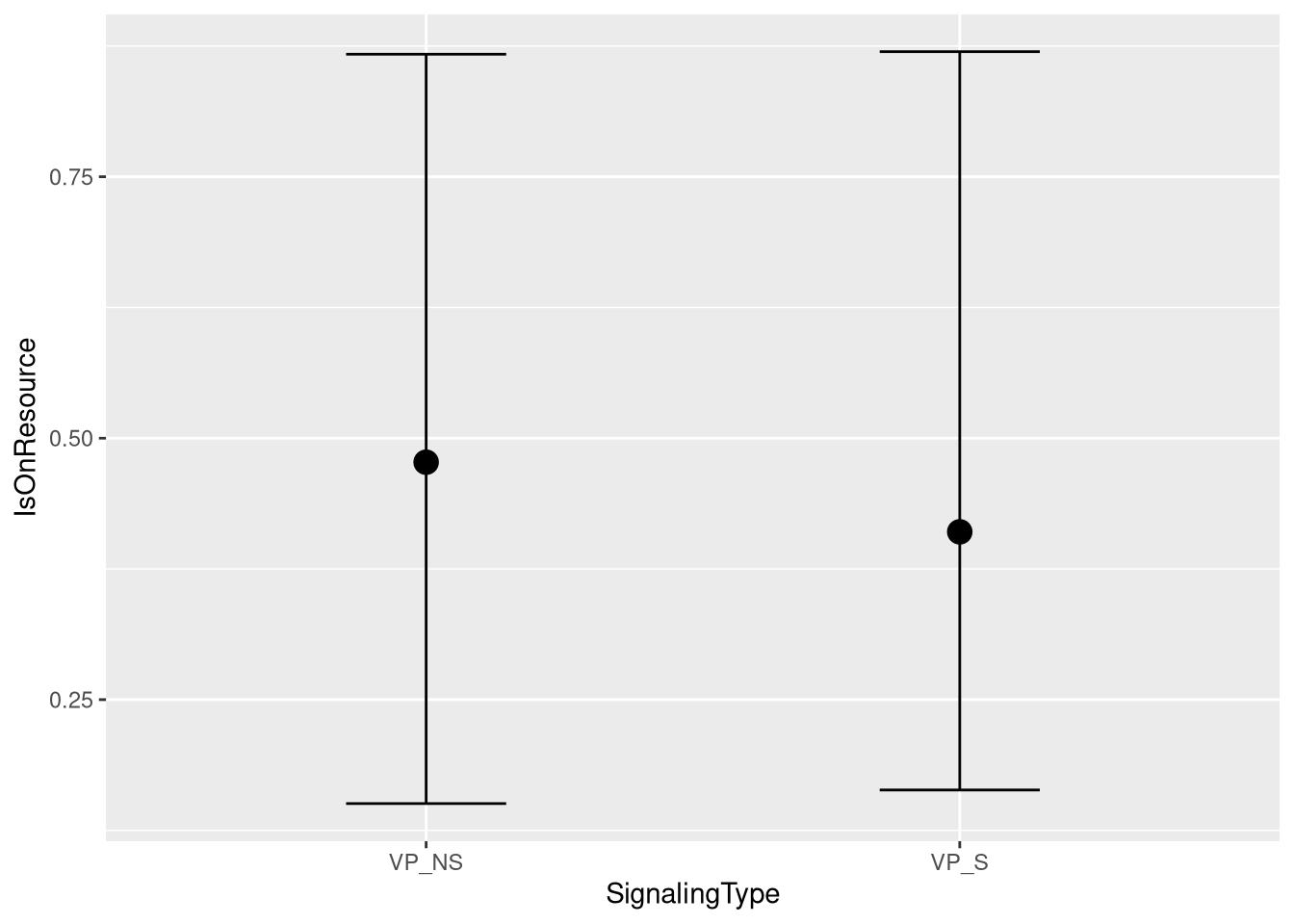
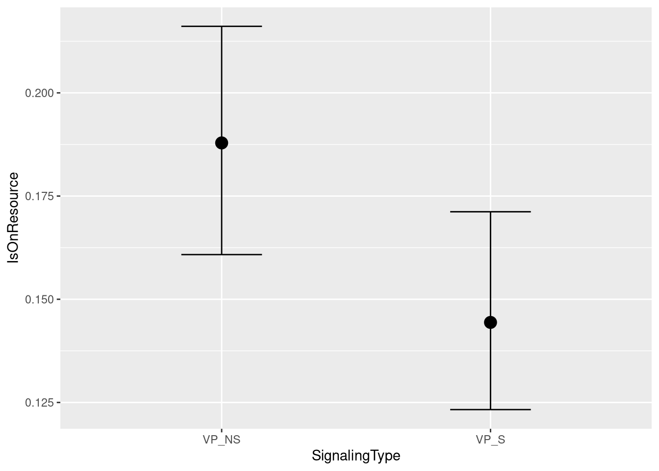
Probability of staying on resource VP
m.events.s.pstay.VP.data <- resource_discoveries_data_vp %>%
  filter(ResourceSpeed == 'slow', PlayerOrderCat == 'first') %>%
  filter(((Timepoint * 10) %% 10 == 0))
m.events.s.pstay.VP.data %>%
group_by(ResourceSpeed, SignalingType) %>%
summarise(UniqueEvents = n_distinct(Event))m.events.s.pstay.VP.formula <- brmsformula(
IsOnResource ~ gp(Timepoint, by = SignalingType),
family = bernoulli(link = "logit")
)m.events.s.pstay.VP.priors <-
prior(normal(0, 1), class = "Intercept") +
prior(inv_gamma(10, 20), class = "lscale", coef = "gpTimepointSignalingTypeVP_NS") +
prior(inv_gamma(10, 20), class = "lscale", coef = "gpTimepointSignalingTypeVP_S") +
prior(normal(0, 0.25), class = "sdgp", lb = 0)Prior predictive checks
m.events.s.pstay.VP.fit_prior <- brm(
  formula = m.events.s.pstay.VP.formula,
  prior   = m.events.s.pstay.VP.priors,
  data    = m.events.s.pstay.VP.data,
  seed    = 42,
  chains  = 4,
  cores   = 4,
  iter    = 2000,
  file = paste0(fits_path, 'resource_discoveries_slow_p_stay_vp_prior.rds'),
  backend = "cmdstanr",
  threads = threading(100),
  control = list(adapt_delta = 0.95),
  save_pars = save_pars(all = TRUE),
  sample_prior = "only"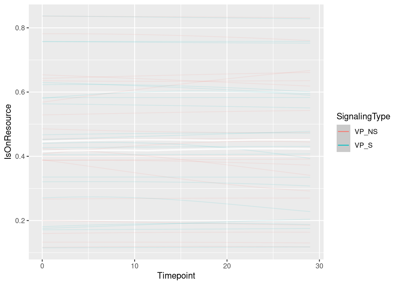
)plot(conditional_effects(m.events.s.pstay.VP.fit_prior, ndraws = 20, spaghetti = TRUE), points = F, ask = F)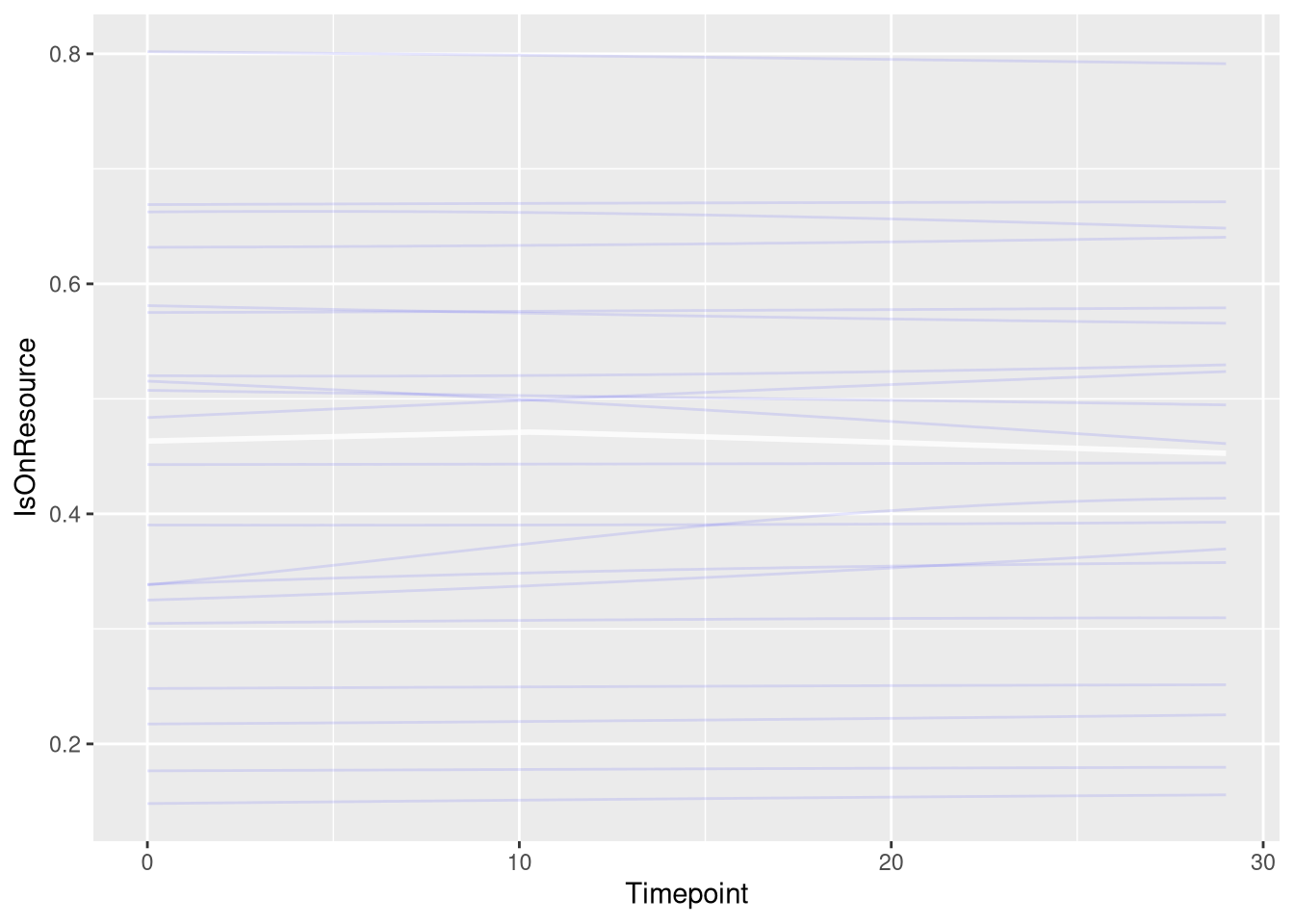
Model fitting
m.events.s.pstay.VP.fit <- brm(
  formula = m.events.s.pstay.VP.formula,
  prior   = m.events.s.pstay.VP.priors,
  data    = m.events.s.pstay.VP.data,
  chains = 4,
  cores = 4,
  seed = 42,
  warmup = 500,
  iter = 2000,
  file = paste0(fits_path, 'resource_discoveries_slow_p_stay_vp.rds'),
  backend = "cmdstanr",
  threads = threading(100),
  control = list(adapt_delta = 0.95),
  save_pars = save_pars(all = TRUE)
)## Family: bernoulli
## Links: mu = logit
## Formula: IsOnResource ~ gp(Timepoint, by = SignalingType)
## Data: m.events.s.pstay.VP.data (Number of observations: 600)
## Draws: 4 chains, each with iter = 2000; warmup = 500; thin = 1;
## total post-warmup draws = 6000
##
## Gaussian Process Hyperparameters:
## Estimate Est.Error l-95% CI u-95% CI Rhat Bulk_ESS Tail_ESS
## sdgp(gpTimepointSignalingTypeVP_NS) 0.84 0.15 0.57 1.16 1.00 6257 4157
## sdgp(gpTimepointSignalingTypeVP_S) 0.41 0.23 0.03 0.86 1.00 1824 1507
## lscale(gpTimepointSignalingTypeVP_NS) 1.08 0.23 0.72 1.59 1.00 6293 4438
## lscale(gpTimepointSignalingTypeVP_S) 1.87 0.68 0.98 3.61 1.00 4962 4628
##
## Regression Coefficients:
## Estimate Est.Error l-95% CI u-95% CI Rhat Bulk_ESS Tail_ESS
## Intercept 1.33 0.41 0.39 2.00 1.00 2468 3402
##
## Draws were sampled using sample(hmc). For each parameter, Bulk_ESS
## and Tail_ESS are effective sample size measures, and Rhat is the potential
## scale reduction factor on split chains (at convergence, Rhat = 1).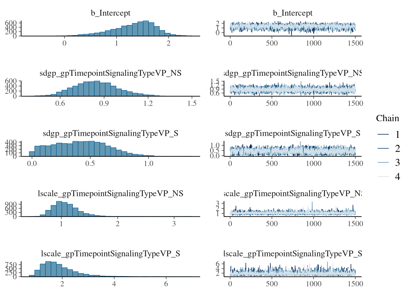
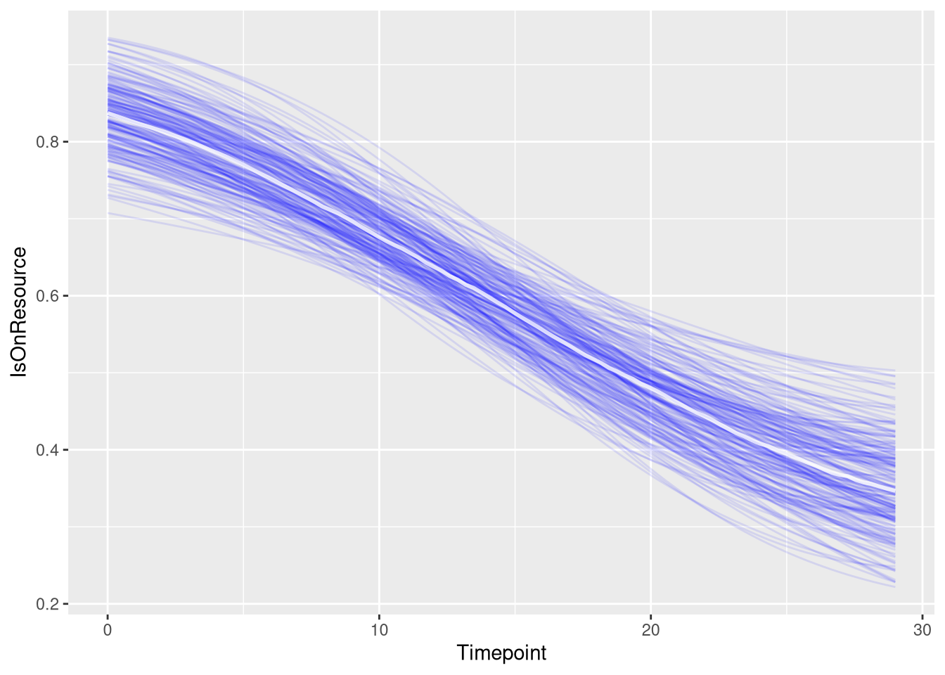
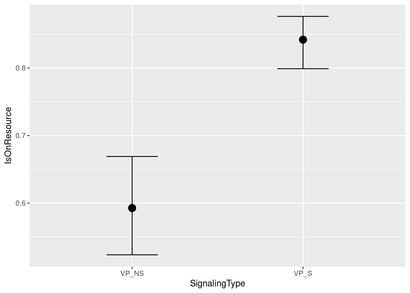
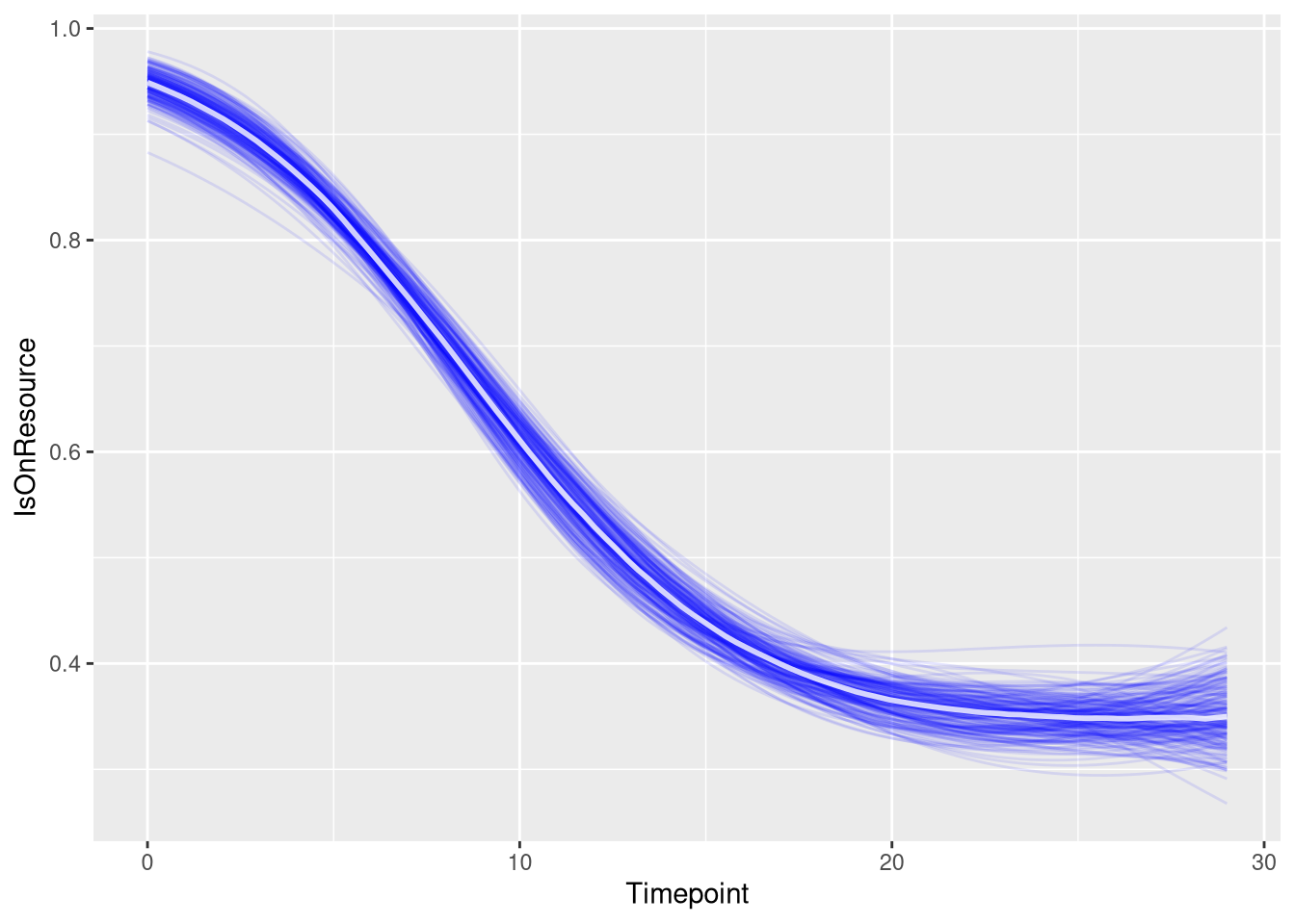
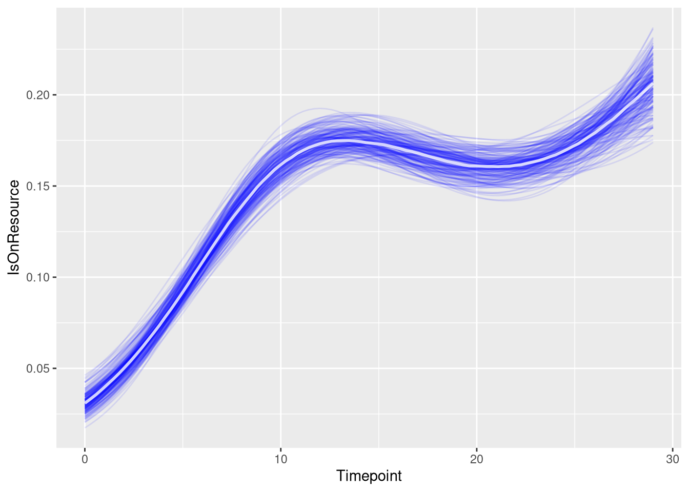
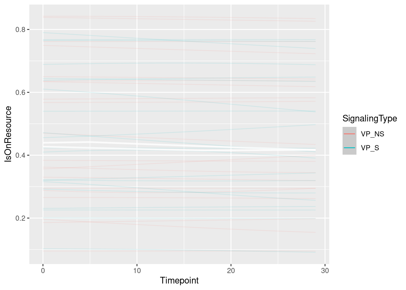
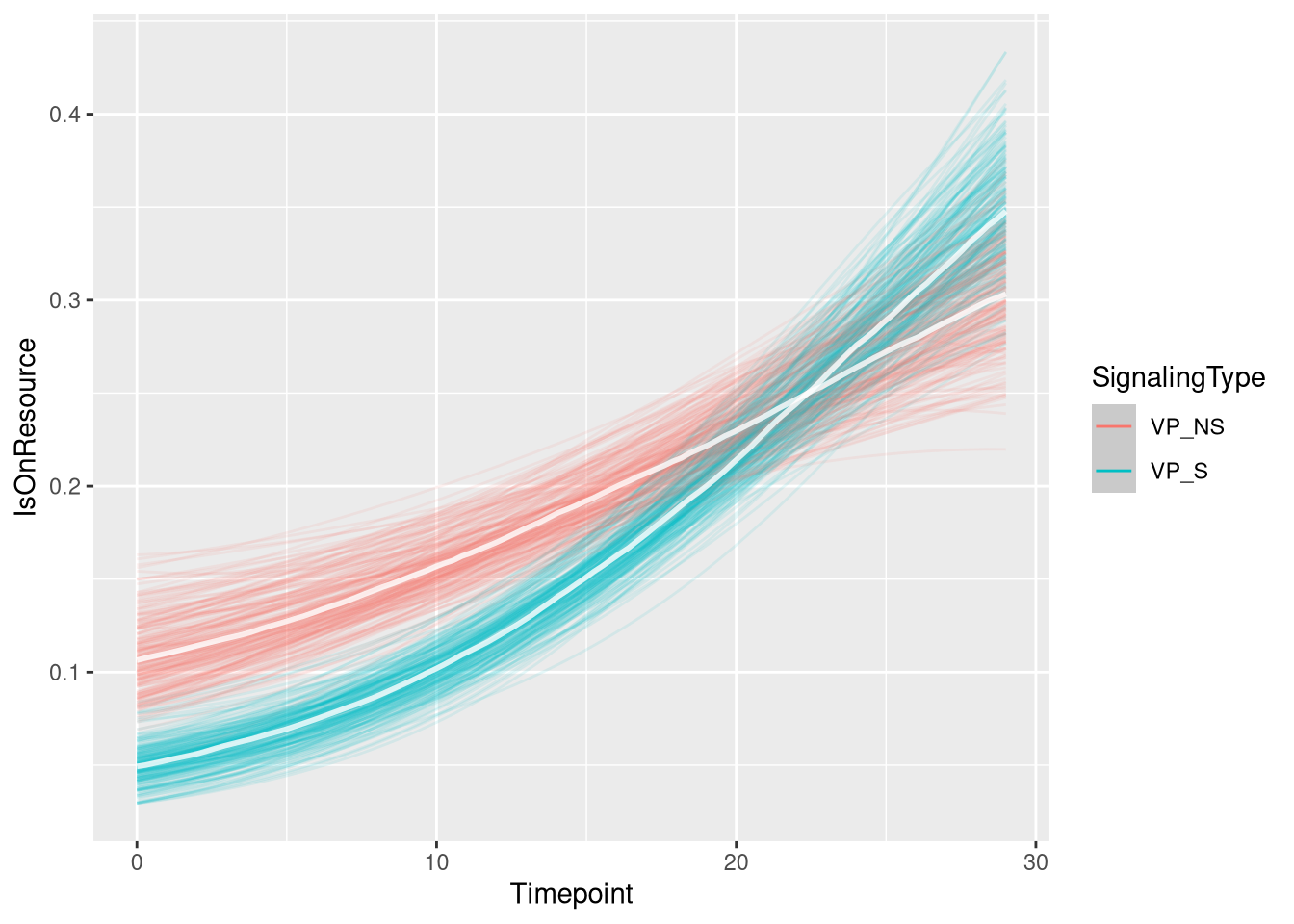
Figure
m.events.s.pstay.VP.draws <- m.events.s.pstay.VP.data %>%
  mutate(SignalingType = factor(SignalingType, levels = c('VP_NS', 'VP_S'))) %>%
  data_grid(Timepoint, SignalingType) %>%
  tidybayes::add_epred_draws(m.events.s.pstay.VP.fit, allow_new_levels = TRUE, re_formula = m.events.s.pstay.VP.formula)
events_slow_p_stay_vp_fig <- m.events.s.pstay.VP.draws %>%
ggplot(aes(x = Timepoint, y = .epred, fill = SignalingType, color = SignalingType)) + # , group = SignalingType
stat_lineribbon(aes(group = paste(group, ...width..)), .width = c(.9), alpha = 1/2) +
theme_clean() +
panel_border() +
theme(legend.position = "none") +
scale_color_manual(breaks = c('VP_NS', 'VP_S'),
aesthetics = c("colour", "fill"),
values = c("#000000", "#DF536B"),
guide = guide_legend(
title = "Signaling",
)
) +
scale_y_continuous(
limits = c(0.15, 1.0),
expand = expansion(mult = c(0, 0))
) +
scale_x_continuous(
limits = c(0, 30),
expand = expansion(mult = c(0, 0))
) +
labs(x = "Time [s]",
y = "P(on resource)")
events_slow_p_stay_vp_fig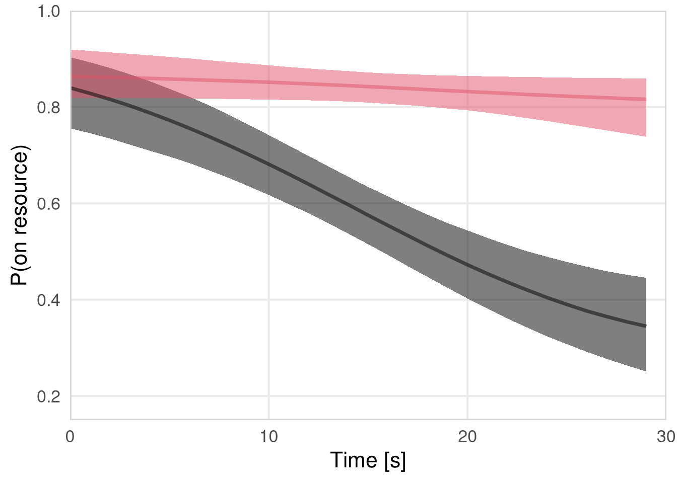
Probability of reaching on resource
m.events.s.reach.data <- resource_discoveries_data %>%
  filter(ResourceSpeed == 'slow', PlayerOrderCat == 'others') %>%
  filter(((Timepoint * 10) %% 10 == 0))


m.events.s.reach.formula <- brmsformula(
  IsOnResource ~ gp(Timepoint, by = SignalingType),
  family = bernoulli(link = "logit")
  )
m.events.s.reach.priors <-
prior(normal(0, 1), class = "Intercept") +
prior(inv_gamma(10, 20), class = "lscale", coef = "gpTimepointSignalingTypeFP") +
prior(inv_gamma(10, 20), class = "lscale", coef = "gpTimepointSignalingTypeNP") +
prior(inv_gamma(10, 20), class = "lscale", coef = "gpTimepointSignalingTypeVP") +
prior(normal(0, 0.25), class = "sdgp", lb = 0)Prior predictive checks
m.events.s.reach.fit_prior <- brm(
  formula = m.events.s.reach.formula,
  prior   = m.events.s.reach.priors,
  data    = m.events.s.reach.data,
  chains  = 4,
  cores   = 4,
  seed    = 42,
  iter    = 2000,
  file = paste0(fits_path, 'resource_discoveries_slow_p_reach_prior.rds'),
  backend = "cmdstanr",
  threads = threading(100),
  control = list(adapt_delta = 0.95),
  save_pars = save_pars(all = TRUE),
  sample_prior = "only"
)plot(conditional_effects(m.events.s.reach.fit_prior, ndraws = 20, spaghetti = TRUE), points = F, ask = F)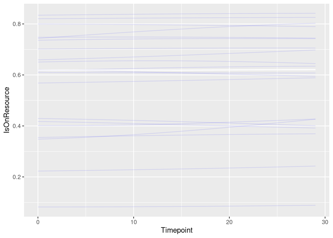
Model fitting
m.events.s.reach.fit <- brm(
  formula = m.events.s.reach.formula,
  prior   = m.events.s.reach.priors,
  data    = m.events.s.reach.data,
  chains = 4,
  cores = 4,
  seed = 42,
  warmup = 500,
  iter = 2000,
  file = paste0(fits_path, 'resource_discoveries_slow_p_reach.rds'),
  backend = "cmdstanr",
  threads = threading(100),
  control = list(adapt_delta = 0.95),
  save_pars = save_pars(all = TRUE)
)## Family: bernoulli
## Links: mu = logit
## Formula: IsOnResource ~ gp(Timepoint, by = SignalingType)
## Data: m.events.s.reach.data (Number of observations: 5340)
## Draws: 4 chains, each with iter = 2000; warmup = 500; thin = 1;
## total post-warmup draws = 6000
##
## Gaussian Process Hyperparameters:
## Estimate Est.Error l-95% CI u-95% CI Rhat Bulk_ESS Tail_ESS
## sdgp(gpTimepointSignalingTypeNP) 0.84 0.14 0.59 1.15 1.00 6627 4427
## sdgp(gpTimepointSignalingTypeVP) 0.81 0.14 0.55 1.12 1.00 5488 3595
## sdgp(gpTimepointSignalingTypeFP) 0.74 0.14 0.48 1.05 1.00 6660 4185
## lscale(gpTimepointSignalingTypeNP) 1.02 0.19 0.71 1.44 1.00 6883 4806
## lscale(gpTimepointSignalingTypeVP) 1.14 0.21 0.79 1.61 1.00 5913 4595
## lscale(gpTimepointSignalingTypeFP) 1.22 0.24 0.83 1.78 1.00 6699 4545
##
## Regression Coefficients:
## Estimate Est.Error l-95% CI u-95% CI Rhat Bulk_ESS Tail_ESS
## Intercept -1.55 0.39 -2.33 -0.81 1.00 2815 3578
##
## Draws were sampled using sample(hmc). For each parameter, Bulk_ESS
## and Tail_ESS are effective sample size measures, and Rhat is the potential
## scale reduction factor on split chains (at convergence, Rhat = 1).
Figure
events_slow_p_reach_fig <- m.events.s.reach.draws %>%
  ggplot(aes(x = Timepoint, y = .epred, fill = SignalingType, color = SignalingType)) +
  stat_lineribbon(aes(group = paste(group, ...width..)), .width = c(.9), alpha = 1/2) +
  theme_nice(legend.pos = "top") +
  scale_color_manual(breaks = c('NP', 'VP', 'FP'),
                     aesthetics = c("colour", "fill"),
                    values = c("#DF536B", "#61D04F", "#2297E6"),
                    guide = guide_legend(
                      title = "Signaling",
                     )
                    ) +
  theme_clean() +
  panel_border() +
  theme(legend.position    = "none") +
  scale_y_continuous(
    limits  = c(0, 0.5),
    expand  = expansion(mult = c(0, 0))
  ) +
  scale_x_continuous(
    limits  = c(0, 30),
    expand  = expansion(mult = c(0, 0))
  ) +
  labs(x = "Time [s]",
       y = "P(on resource)")

events_slow_p_reach_fig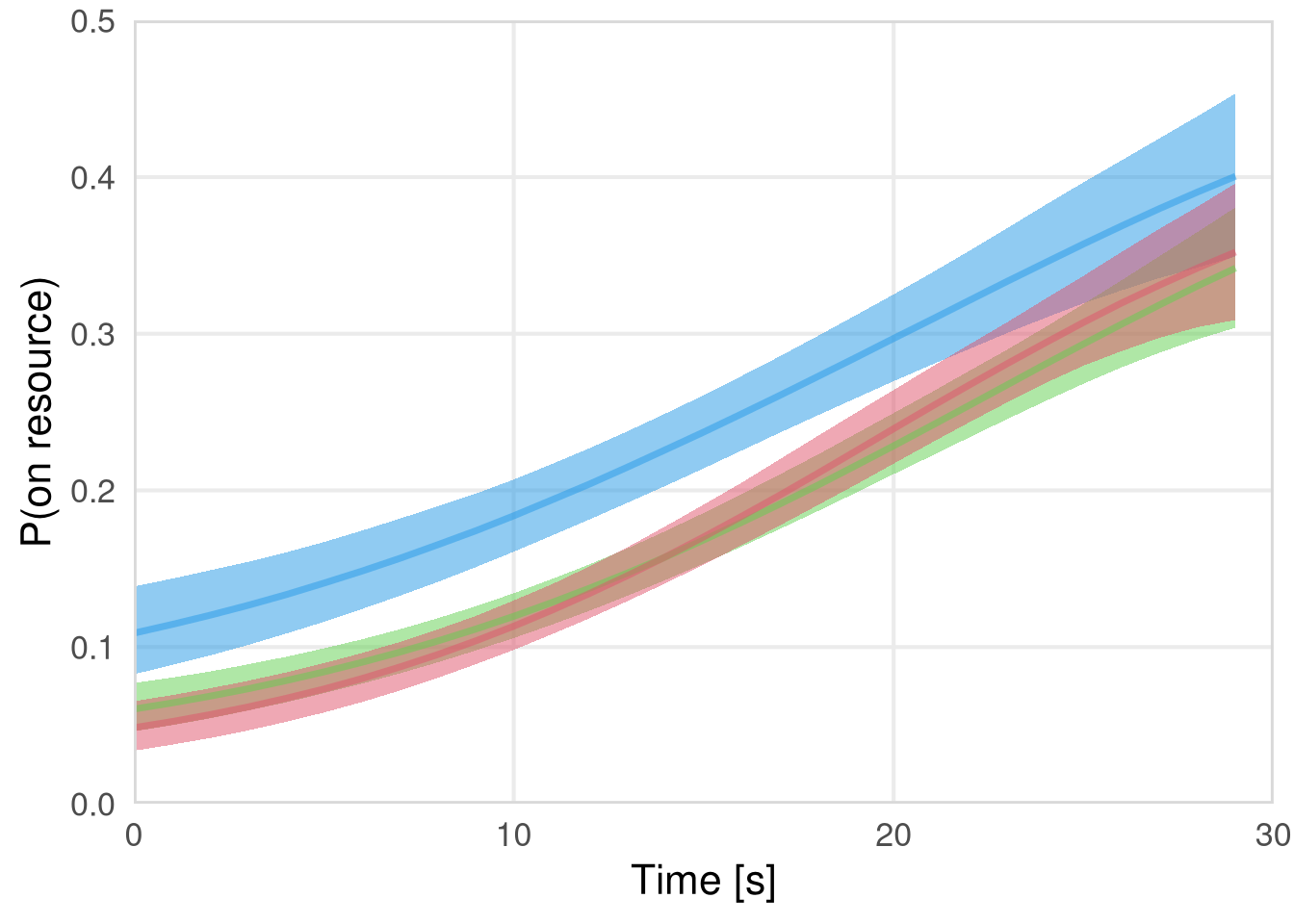
Probability of reaching resource VP
m.events.s.reach.VP.data <- resource_discoveries_data_vp %>%
  filter(ResourceSpeed == 'slow', PlayerOrderCat == 'others') %>%
  filter(((Timepoint * 10) %% 10 == 0))


m.events.s.reach.VP.formula <- brmsformula(
  IsOnResource ~ gp(Timepoint, by = SignalingType),
  family = bernoulli(link = "logit")
  )
m.events.s.reach.VP.priors <-
prior(normal(0, 1), class = "Intercept") +
prior(inv_gamma(10, 20), class = "lscale", coef = "gpTimepointSignalingTypeVP_NS") +
prior(inv_gamma(10, 20), class = "lscale", coef = "gpTimepointSignalingTypeVP_S") +
prior(normal(0, 0.25), class = "sdgp", lb = 0)Prior predictive checks
m.events.s.reach.VP.fit_prior <- brm(
  formula = m.events.s.reach.VP.formula,
  prior   = m.events.s.reach.VP.priors,
  data    = m.events.s.reach.VP.data,
  chains  = 4,
  cores   = 4,
  seed    = 42,
  iter    = 2000,
  file = paste0(fits_path, 'resource_discoveries_slow_p_reach_vp_prior.rds'),
  backend = "cmdstanr",
  threads = threading(100),
  control = list(adapt_delta = 0.95),
  save_pars = save_pars(all = TRUE),
  sample_prior = "only"
)plot(conditional_effects(m.events.s.reach.VP.fit_prior, ndraws = 20, spaghetti = TRUE), points = F, ask = F)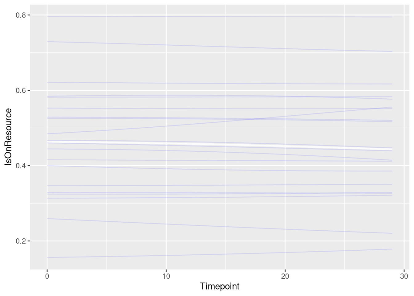
Model fitting
m.events.s.reach.VP.fit <- brm(
  formula = m.events.s.reach.VP.formula,
  prior   = m.events.s.reach.VP.priors,
  data    = m.events.s.reach.VP.data,
  chains = 4,
  cores = 4,
  seed = 42,
  warmup = 500,
  iter = 2000,
  file = paste0(fits_path, 'resource_discoveries_slow_p_reach_vp.rds'),
  backend = "cmdstanr",
  threads = threading(100),
  control = list(adapt_delta = 0.95),
  save_pars = save_pars(all = TRUE)
)## Family: bernoulli
## Links: mu = logit
## Formula: IsOnResource ~ gp(Timepoint, by = SignalingType)
## Data: m.events.s.reach.VP.data (Number of observations: 2280)
## Draws: 4 chains, each with iter = 2000; warmup = 500; thin = 1;
## total post-warmup draws = 6000
##
## Gaussian Process Hyperparameters:
## Estimate Est.Error l-95% CI u-95% CI Rhat Bulk_ESS Tail_ESS
## sdgp(gpTimepointSignalingTypeVP_NS) 0.67 0.15 0.40 0.98 1.00 7994 4006
## sdgp(gpTimepointSignalingTypeVP_S) 0.84 0.14 0.58 1.14 1.00 6775 4354
## lscale(gpTimepointSignalingTypeVP_NS) 1.32 0.30 0.85 2.02 1.00 9569 4397
## lscale(gpTimepointSignalingTypeVP_S) 1.09 0.20 0.76 1.54 1.00 7675 4609
##
## Regression Coefficients:
## Estimate Est.Error l-95% CI u-95% CI Rhat Bulk_ESS Tail_ESS
## Intercept -1.40 0.45 -2.26 -0.54 1.00 4283 4391
##
## Draws were sampled using sample(hmc). For each parameter, Bulk_ESS
## and Tail_ESS are effective sample size measures, and Rhat is the potential
## scale reduction factor on split chains (at convergence, Rhat = 1).
Figure
m.events.s.reach.VP.draws <- m.events.s.reach.VP.data %>%
  mutate(SignalingType = factor(SignalingType, levels = c('VP_NS', 'VP_S'))) %>%
  data_grid(Timepoint, SignalingType) %>%
  tidybayes::add_epred_draws(m.events.s.reach.VP.fit, allow_new_levels = TRUE, re_formula = m.events.s.reach.VP.formula)
events_slow_p_reach_vp_fig <- m.events.s.reach.VP.draws %>%
ggplot(aes(x = Timepoint, y = .epred, fill = SignalingType, color = SignalingType)) +
stat_lineribbon(aes(group = paste(group, ...width..)), .width = c(.9), alpha = 1/2) +
theme_nice(legend.pos = 'top') +
scale_color_manual(breaks = c('VP_NS', 'VP_S'),
aesthetics = c("colour", "fill"),
values = c("#000000", "#DF536B"),
guide = guide_legend(
title = "Signaling",
)
) +
theme_clean() +
panel_border() +
theme(legend.position = "none") +
scale_y_continuous(
limits = c(0, 0.5),
expand = expansion(mult = c(0, 0))
) +
scale_x_continuous(
limits = c(0, 30),
expand = expansion(mult = c(0, 0))
) +
labs(x = "Time [s]",
y = "P(on resource)")
events_slow_p_reach_vp_fig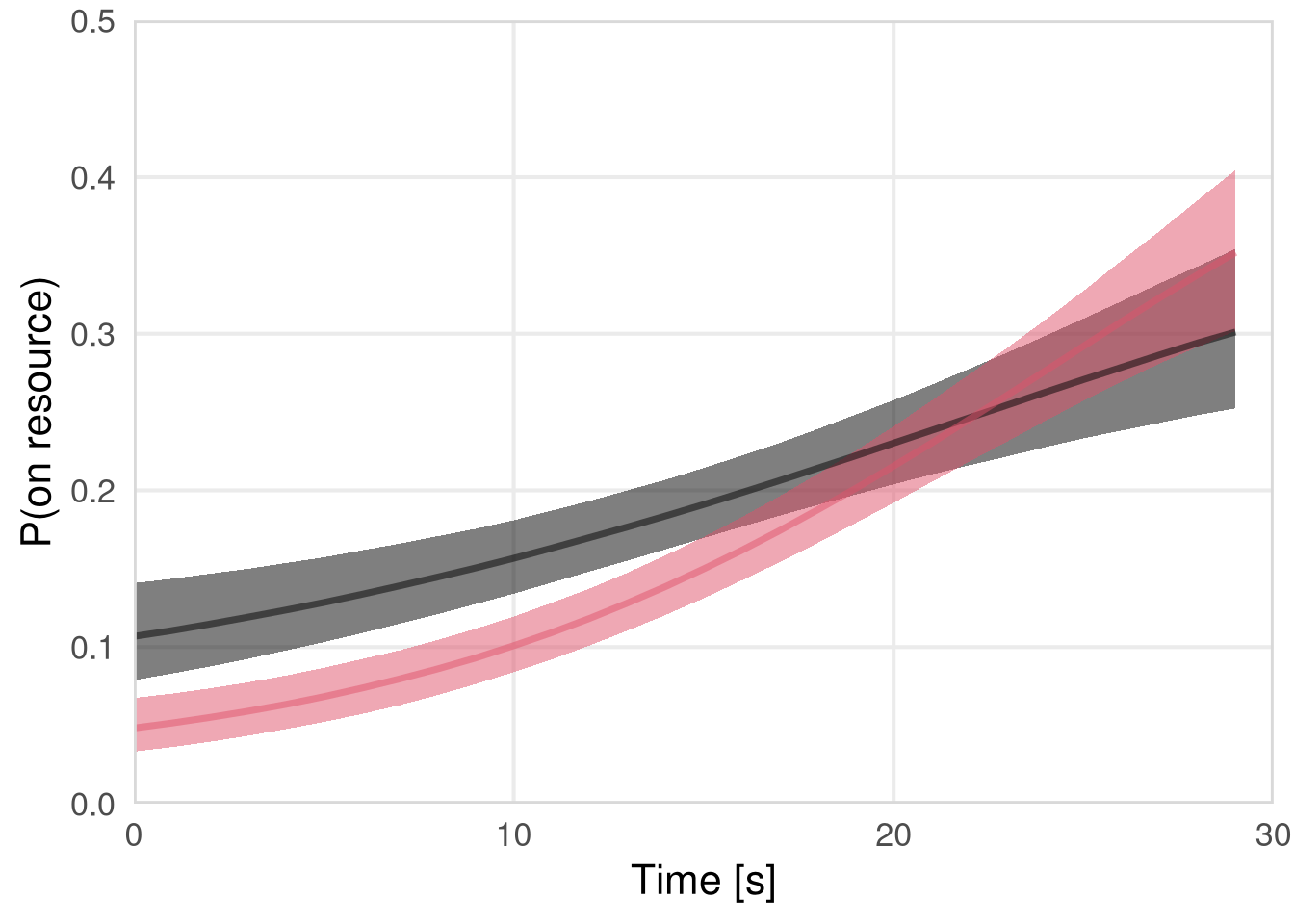
Out degree
m.events.s.OutDegree.data <- resource_discoveries_data %>%
  filter(ResourceSpeed == 'slow', SignalingType != 'A', PlayerOrderCat == 'others') %>%
  filter(((Timepoint * 10) %% 10 == 0))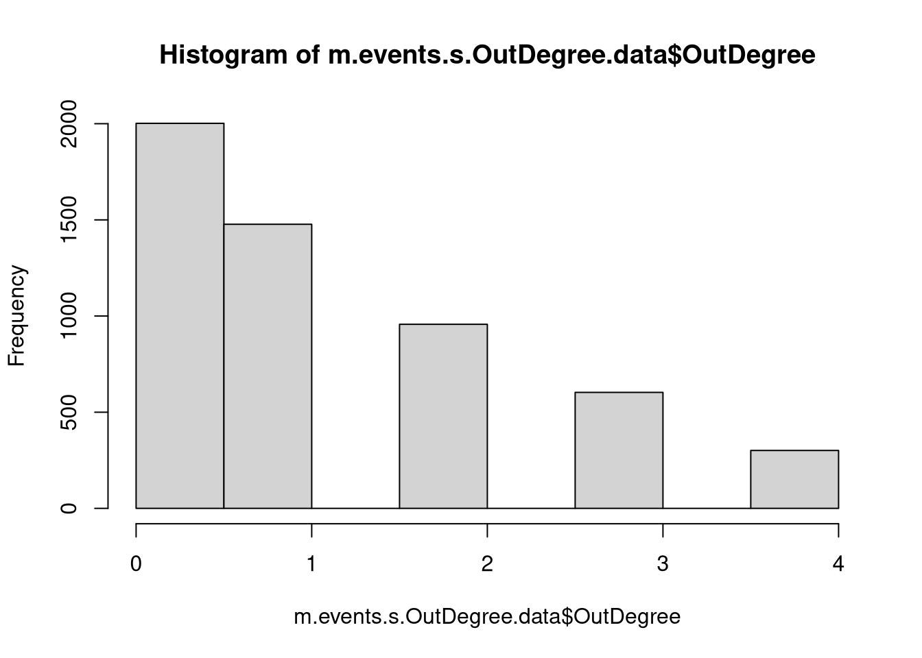
m.events.s.OutDegree.formula <- brmsformula(
  OutDegree ~ gp(Timepoint, by = SignalingType),
  family = poisson(link = "log")
  )
m.events.s.OutDegree.priors <-
prior(normal(0, 1), class = "Intercept") +
prior(inv_gamma(10, 20), class = "lscale", coef = "gpTimepointSignalingTypeFP") +
prior(inv_gamma(10, 20), class = "lscale", coef = "gpTimepointSignalingTypeNP") +
prior(inv_gamma(10, 20), class = "lscale", coef = "gpTimepointSignalingTypeVP") +
prior(normal(0, 0.25), class = "sdgp", lb = 0)Prior predictive checks
m.events.s.OutDegree.fit_prior <- brm(
  formula = m.events.s.OutDegree.formula,
  prior   = m.events.s.OutDegree.priors,
  data    = m.events.s.OutDegree.data,
  chains  = 4,
  cores   = 4,
  seed    = 42,
  iter    = 2000,
  file = paste0(fits_path, 'resource_discoveries_slow_out_degree_prior.rds'),
  backend = "cmdstanr",
  threads = threading(100),
  control = list(adapt_delta = 0.95),
  save_pars = save_pars(all = TRUE),
  sample_prior = "only"
)plot(conditional_effects(m.events.s.OutDegree.fit_prior, ndraws = 20, spaghetti = TRUE), points = F, ask = F)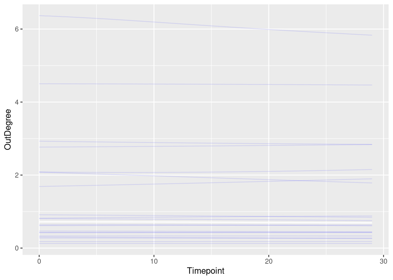
Model fitting
m.events.s.OutDegree.fit <- brm(
  formula = m.events.s.OutDegree.formula,
  prior   = m.events.s.OutDegree.priors,
  data    = m.events.s.OutDegree.data,
  chains = 4,
  cores = 4,
  seed = 42,
  warmup = 500,
  iter = 2000,
  file = paste0(fits_path, 'resource_discoveries_slow_out_degree.rds'),
  backend = "cmdstanr",
  threads = threading(100),
  control = list(adapt_delta = 0.95),
  save_pars = save_pars(all = TRUE)
)## Family: poisson
## Links: mu = log
## Formula: OutDegree ~ gp(Timepoint, by = SignalingType)
## Data: m.events.s.OutDegree.data (Number of observations: 5340)
## Draws: 4 chains, each with iter = 2000; warmup = 500; thin = 1;
## total post-warmup draws = 6000
##
## Gaussian Process Hyperparameters:
## Estimate Est.Error l-95% CI u-95% CI Rhat Bulk_ESS Tail_ESS
## sdgp(gpTimepointSignalingTypeNP) 0.28 0.14 0.05 0.62 1.00 3611 2232
## sdgp(gpTimepointSignalingTypeVP) 0.42 0.13 0.21 0.70 1.00 7049 4051
## sdgp(gpTimepointSignalingTypeFP) 0.47 0.13 0.26 0.77 1.00 7482 4309
## lscale(gpTimepointSignalingTypeNP) 1.97 0.67 1.06 3.58 1.00 10089 4278
## lscale(gpTimepointSignalingTypeVP) 1.75 0.47 1.05 2.85 1.00 9365 4250
## lscale(gpTimepointSignalingTypeFP) 1.47 0.38 0.91 2.37 1.00 10616 5036
##
## Regression Coefficients:
## Estimate Est.Error l-95% CI u-95% CI Rhat Bulk_ESS Tail_ESS
## Intercept 0.07 0.18 -0.30 0.42 1.00 3498 3643
##
## Draws were sampled using sample(hmc). For each parameter, Bulk_ESS
## and Tail_ESS are effective sample size measures, and Rhat is the potential
## scale reduction factor on split chains (at convergence, Rhat = 1).Model diagnostics
m.events.s.OutDegree.me <- conditional_effects(
  m.events.s.OutDegree.fit, ndraws = 200, spaghetti = TRUE)

plot(m.events.s.OutDegree.me, ask = FALSE, points = F)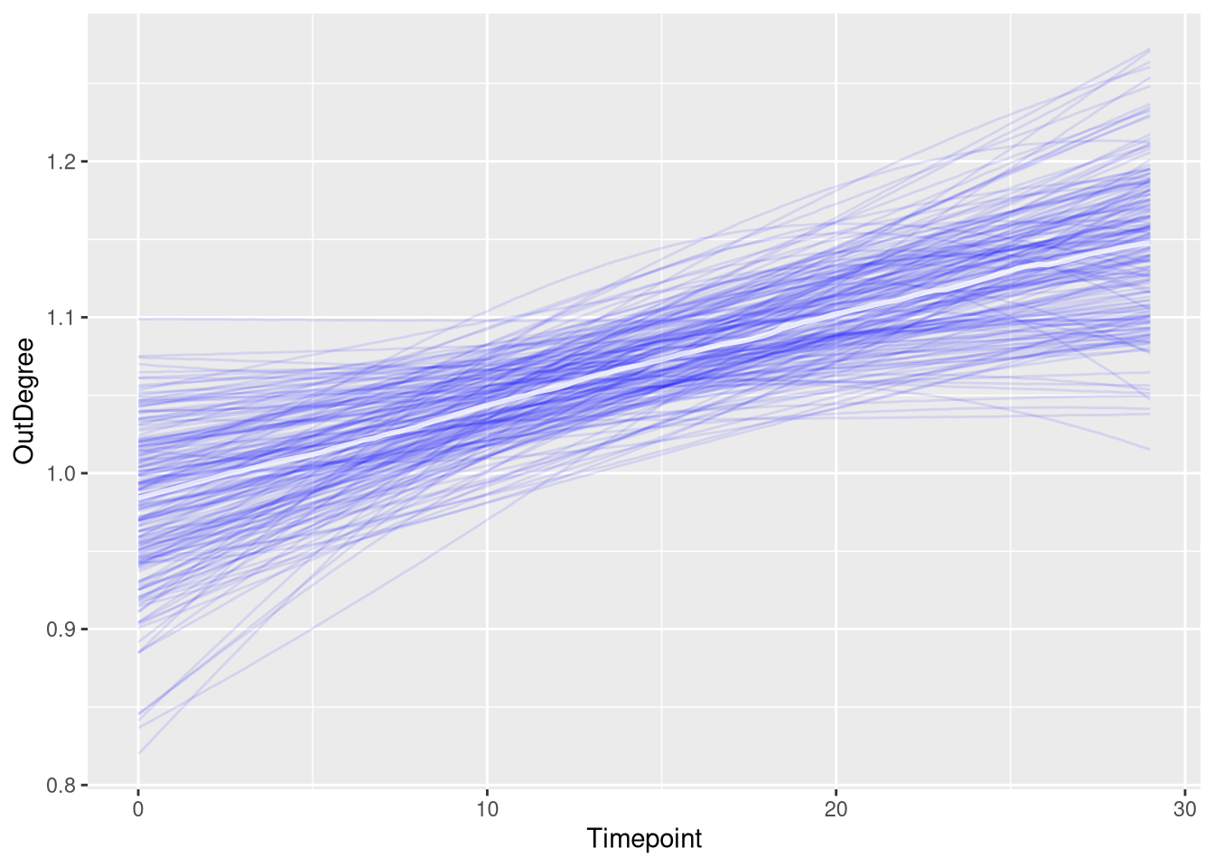
m.events.s.OutDegree.draws <- m.events.s.OutDegree.data %>%
  mutate(SignalingType = factor(SignalingType, levels = c('NP', 'VP', 'FP'))) %>%
  data_grid(Timepoint, SignalingType) %>%
  tidybayes::add_epred_draws(m.events.s.OutDegree.fit, allow_new_levels = TRUE,
                             re_formula = m.events.s.OutDegree.formula)
Figure
events_slow_outdegree_fig <- m.events.s.OutDegree.draws %>%
  ggplot(aes(x = Timepoint, y = .epred, fill = SignalingType, color = SignalingType)) +
  stat_lineribbon(aes(group = paste(group, ...width..)), .width = c(.9), alpha = 1/2) +
  theme_nice(legend.pos = 'none') +
  scale_color_manual(breaks = c('NP', 'VP', 'FP'),
                     aesthetics = c("colour", "fill"),
                    values = c("#DF536B", "#61D04F", "#2297E6"),
                    guide = guide_legend(
                      title = "Signaling",
                     )
                    ) +
  theme_clean() +
  panel_border() +
  theme(legend.position    = "none") +
  scale_x_continuous(
    limits  = c(0, 30),
    expand  = expansion(mult = c(0, 0))
  ) +
  labs(x = "Time [s]",
       y = "Out Degree")


events_slow_outdegree_fig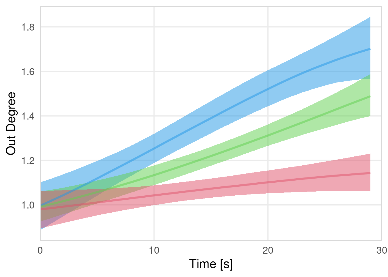
Out degree (Discoverer)
m.events.s.OutDegree.Discoverer.data <- resource_discoveries_data %>%
  filter(ResourceSpeed == 'slow', SignalingType != 'A', PlayerOrderCat == 'first') %>%
  filter(((Timepoint * 10) %% 10 == 0))
m.events.s.OutDegree.Discoverer.formula <- brmsformula(
  OutDegree ~ gp(Timepoint, by = SignalingType),
  family = poisson(link = "log")
  )
m.events.s.OutDegree.Discoverer.priors <-
prior(normal(0, 1), class = "Intercept") +
prior(inv_gamma(10, 20), class = "lscale", coef = "gpTimepointSignalingTypeFP") +
prior(inv_gamma(10, 20), class = "lscale", coef = "gpTimepointSignalingTypeNP") +
prior(inv_gamma(10, 20), class = "lscale", coef = "gpTimepointSignalingTypeVP") +
prior(normal(0, 0.25), class = "sdgp", lb = 0)Prior predictive checks
m.events.s.OutDegree.Discoverer.fit_prior <- brm(
  formula = m.events.s.OutDegree.Discoverer.formula,
  prior   = m.events.s.OutDegree.Discoverer.priors,
  data    = m.events.s.OutDegree.Discoverer.data,
  chains  = 4,
  cores   = 4,
  seed    = 42,
  iter    = 2000,
  file = paste0(fits_path, 'resource_discoveries_slow_out_degree_discoverer_prior.rds'),
  backend = "cmdstanr",
  threads = threading(100),
  control = list(adapt_delta = 0.95),
  save_pars = save_pars(all = TRUE),
  sample_prior = "only"
)plot(conditional_effects(m.events.s.OutDegree.Discoverer.fit_prior, ndraws = 20, spaghetti = TRUE), points = F, ask = F)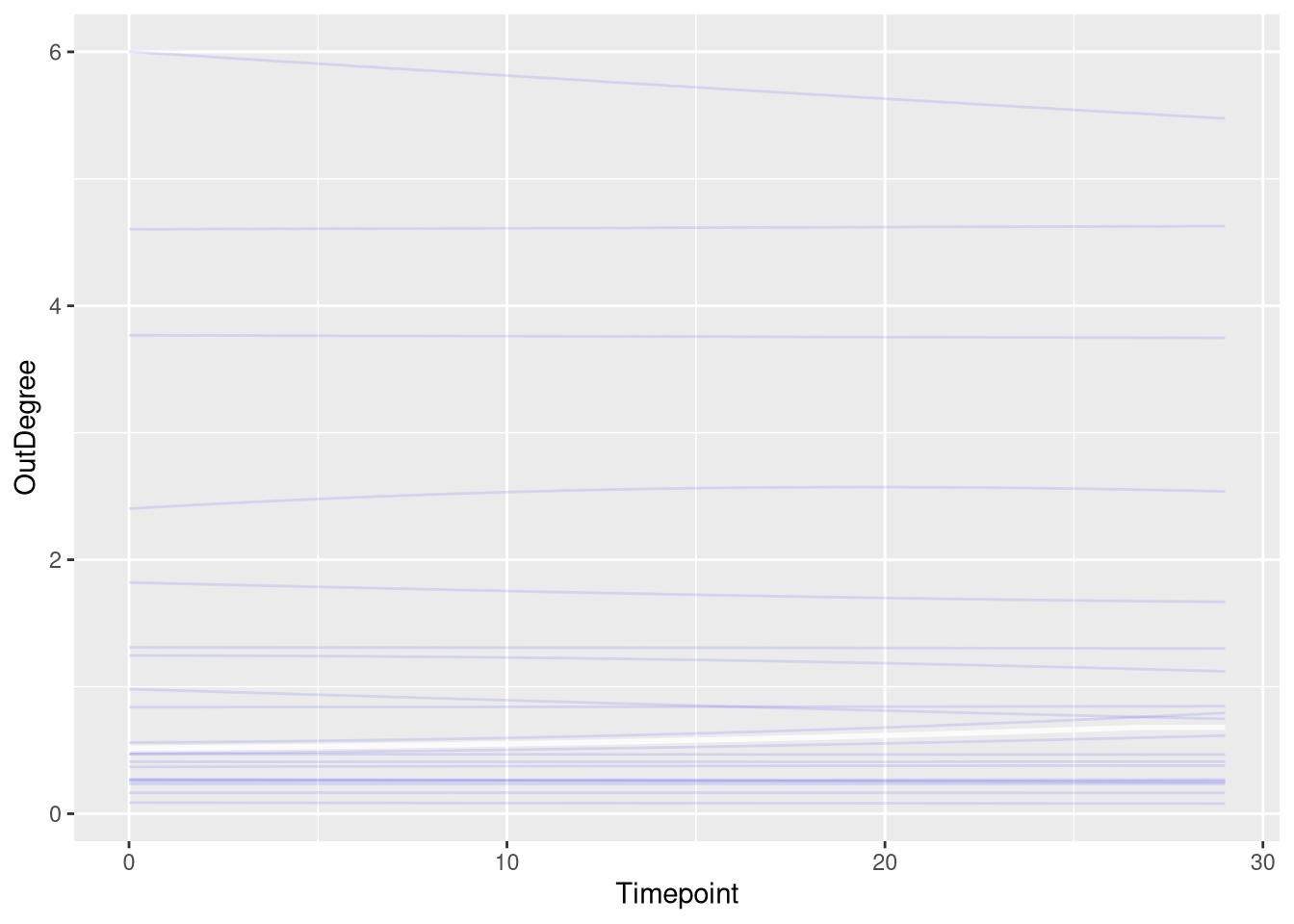
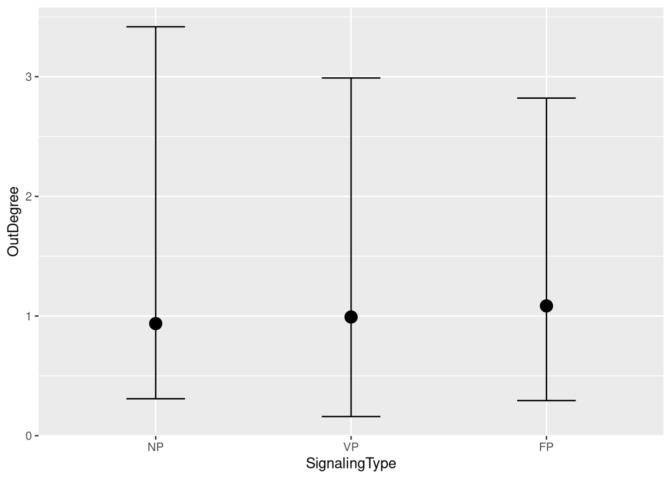
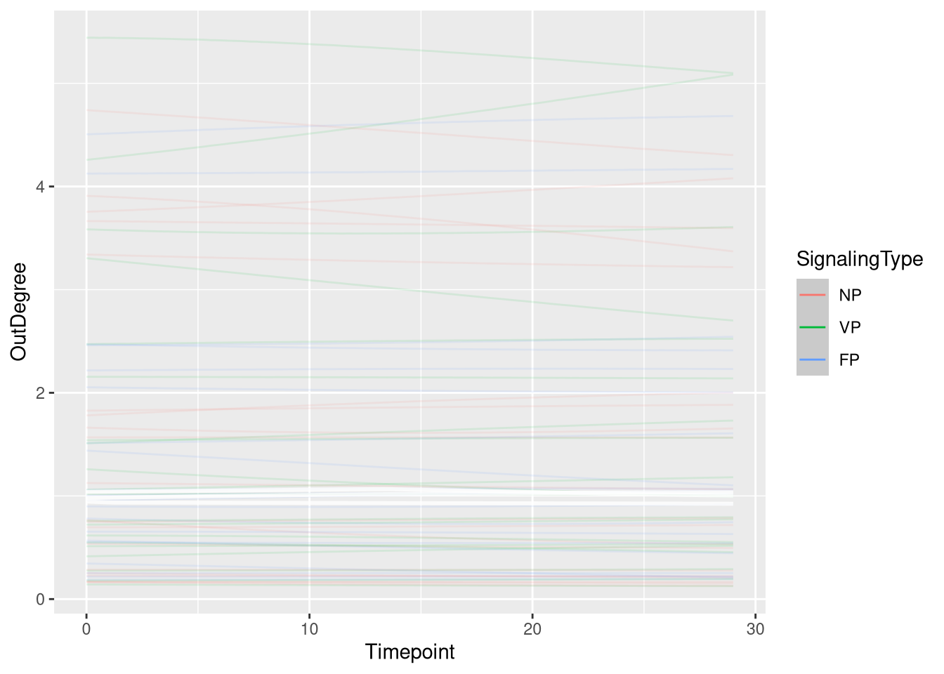
Model fitting
m.events.s.OutDegree.Discoverer.fit <- brm(
  formula = m.events.s.OutDegree.Discoverer.formula,
  prior   = m.events.s.OutDegree.Discoverer.priors,
  data    = m.events.s.OutDegree.Discoverer.data,
  chains = 4,
  cores = 4,
  seed = 42,
  warmup = 500,
  iter = 2000,
  file = paste0(fits_path, 'resource_discoveries_slow_out_degree_discoverer.rds'),
  backend = "cmdstanr",
  threads = threading(100),
  control = list(adapt_delta = 0.95),
  save_pars = save_pars(all = TRUE)
)## Family: poisson
## Links: mu = log
## Formula: OutDegree ~ gp(Timepoint, by = SignalingType)
## Data: m.events.s.OutDegree.Discovererdata (Number of observations: 1380)
## Draws: 4 chains, each with iter = 2000; warmup = 500; thin = 1;
## total post-warmup draws = 6000
##
## Gaussian Process Hyperparameters:
## Estimate Est.Error l-95% CI u-95% CI Rhat Bulk_ESS Tail_ESS
## sdgp(gpTimepointSignalingTypeNP) 0.30 0.17 0.02 0.66 1.00 2380 2376
## sdgp(gpTimepointSignalingTypeVP) 0.51 0.16 0.23 0.87 1.00 4587 3996
## sdgp(gpTimepointSignalingTypeFP) 0.58 0.15 0.31 0.90 1.00 4918 3802
## lscale(gpTimepointSignalingTypeNP) 1.94 0.71 0.98 3.70 1.00 6513 4259
## lscale(gpTimepointSignalingTypeVP) 1.39 0.45 0.72 2.44 1.00 5540 4173
## lscale(gpTimepointSignalingTypeFP) 1.27 0.34 0.77 2.06 1.00 6388 4734
##
## Regression Coefficients:
## Estimate Est.Error l-95% CI u-95% CI Rhat Bulk_ESS Tail_ESS
## Intercept -0.23 0.24 -0.81 0.15 1.00 1778 2196
##
## Draws were sampled using sample(hmc). For each parameter, Bulk_ESS
## and Tail_ESS are effective sample size measures, and Rhat is the potential
## scale reduction factor on split chains (at convergence, Rhat = 1).Model diagnostics
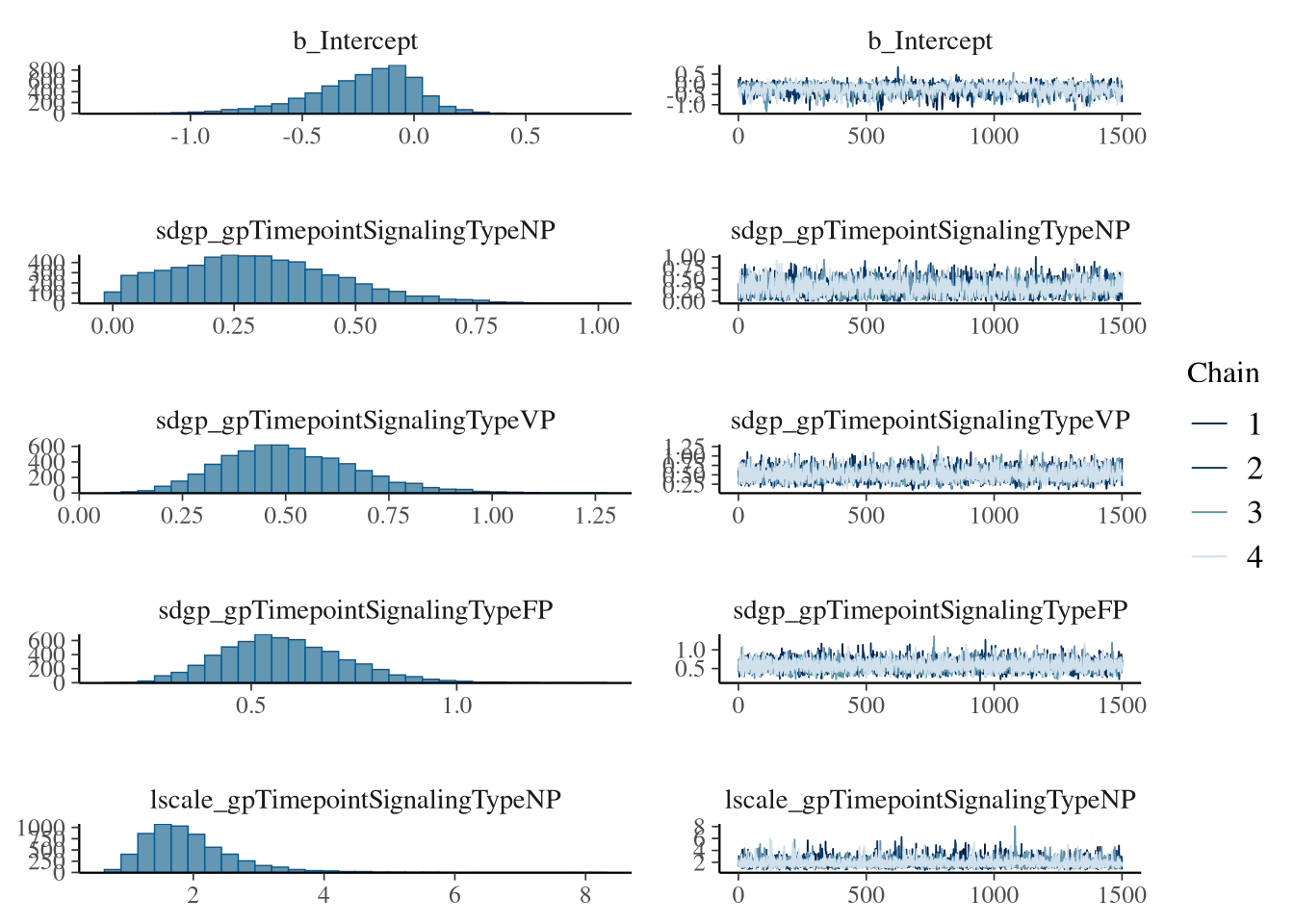
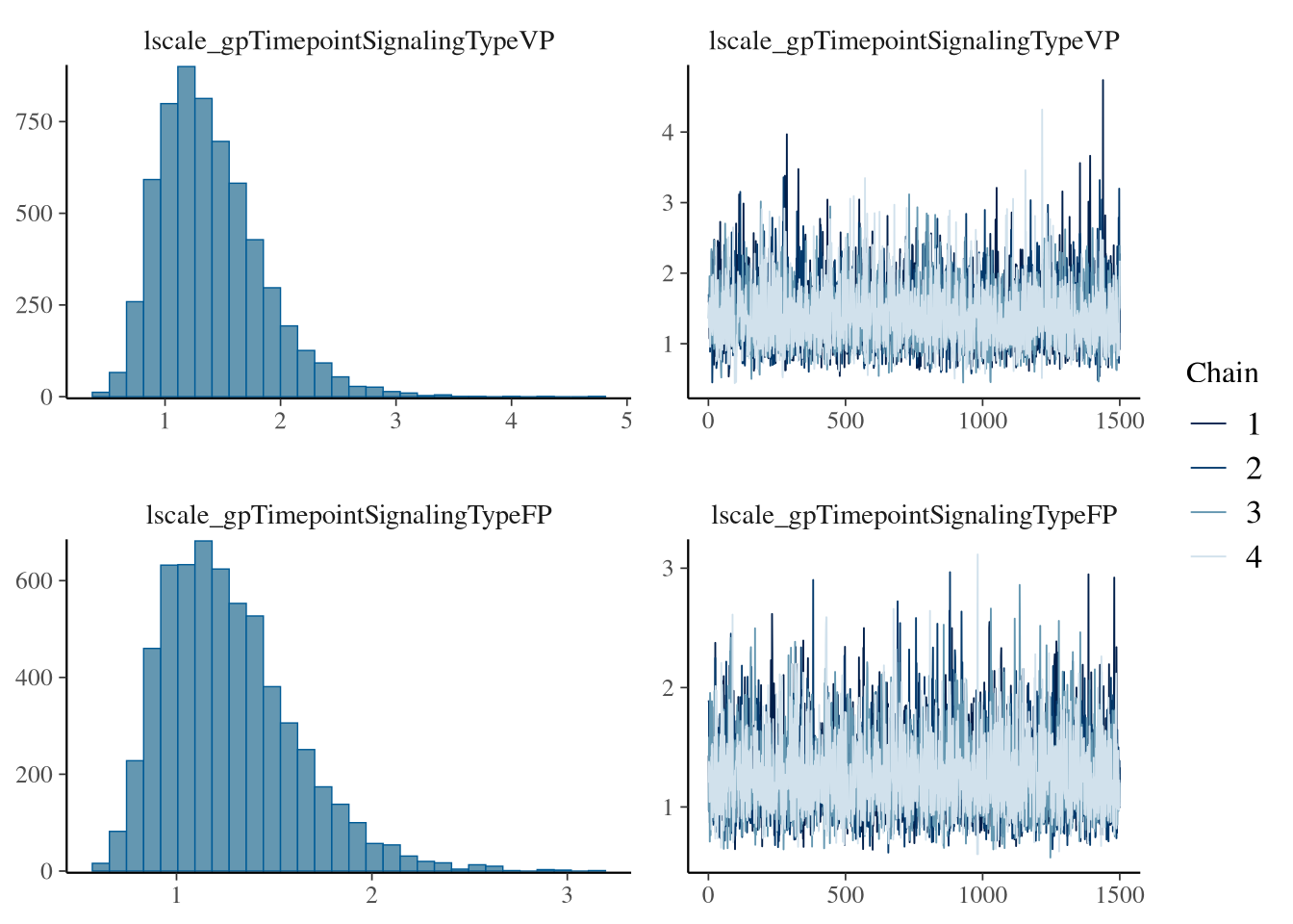
m.events.s.OutDegree.Discoverer.me <- conditional_effects(
  m.events.s.OutDegree.Discoverer.fit, ndraws = 200, spaghetti = TRUE)

plot(m.events.s.OutDegree.Discoverer.me, ask = FALSE, points = F)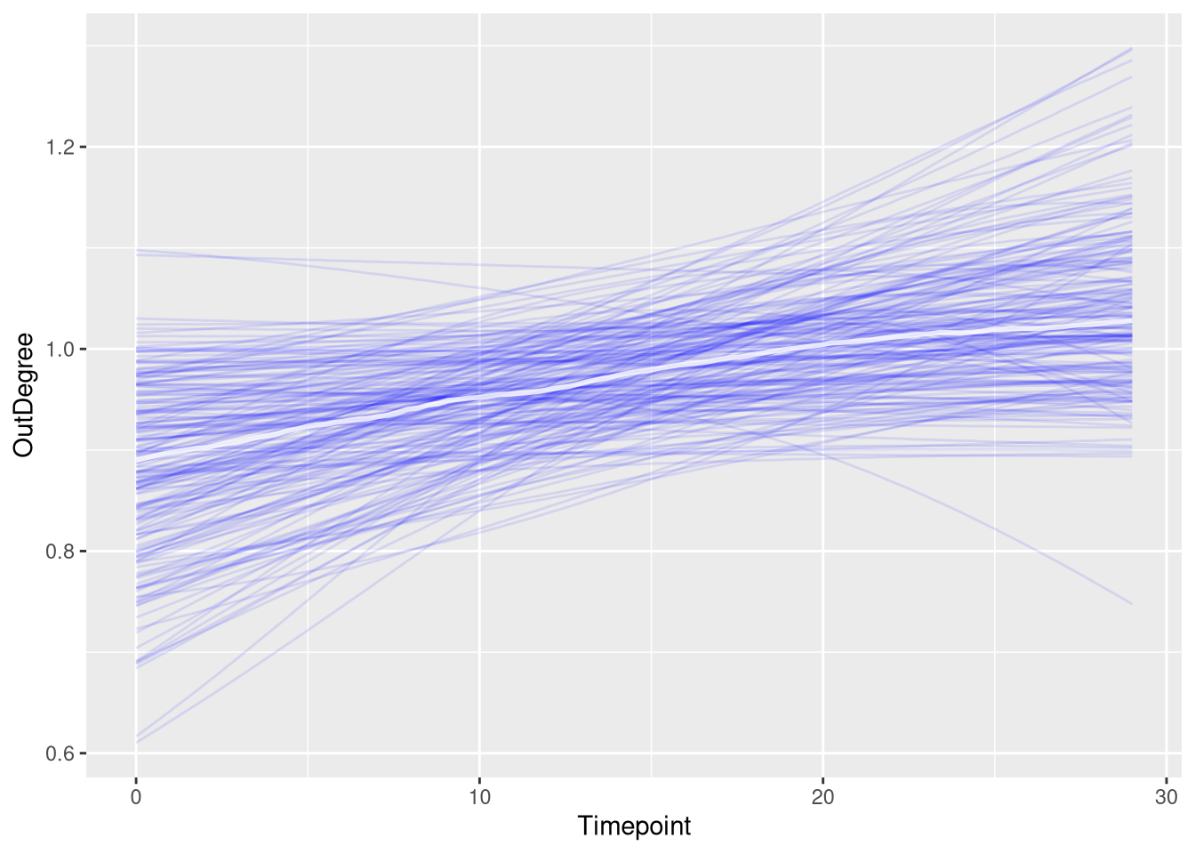
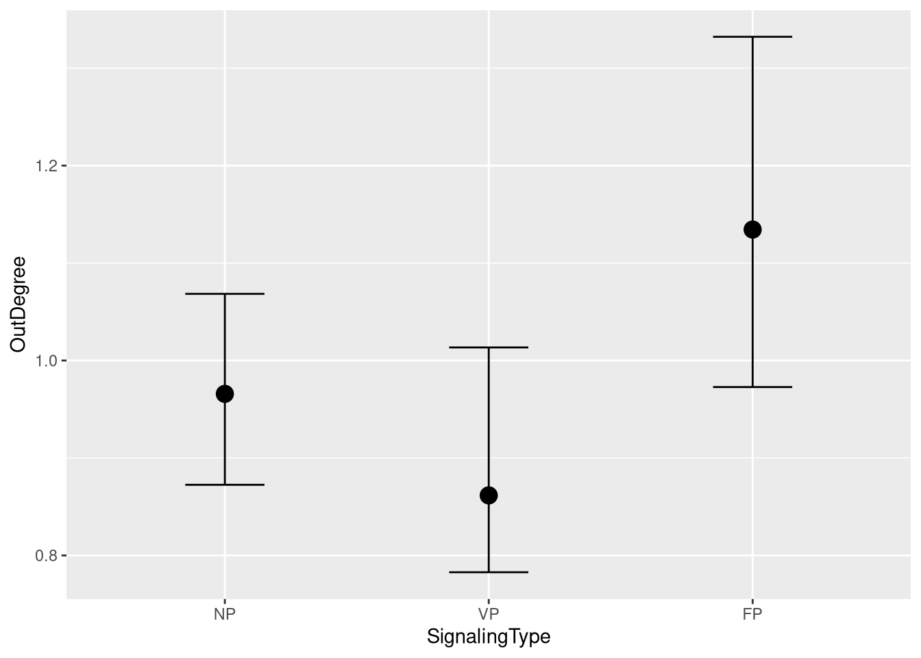
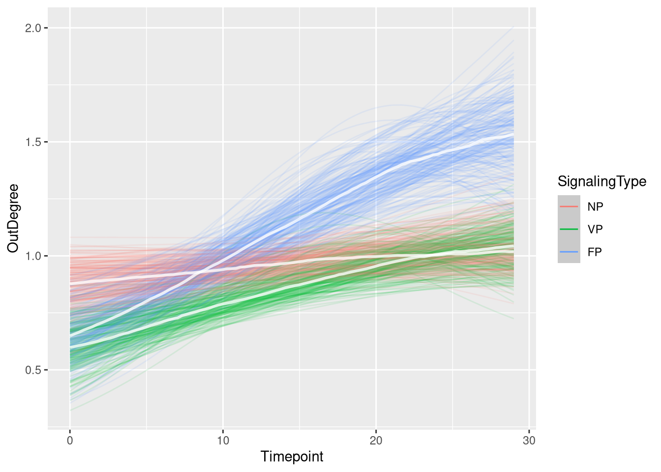
m.events.s.OutDegree.Discoverer.draws <- m.events.s.OutDegree.Discoverer.data %>%
  mutate(SignalingType = factor(SignalingType, levels = c('NP', 'VP', 'FP'))) %>%
  data_grid(Timepoint, SignalingType) %>%
  tidybayes::add_epred_draws(m.events.s.OutDegree.Discoverer.fit, allow_new_levels = TRUE,
                             re_formula = m.events.s.OutDegree.Discoverer.formula)
Figure
events_slow_outdegree_discoverer_fig <- m.events.s.OutDegree.Discoverer.draws %>%
  ggplot(aes(x = Timepoint, y = .epred, fill = SignalingType, color = SignalingType)) +
  stat_lineribbon(aes(group = paste(group, ...width..)), .width = c(.9), alpha = 1/2) +
  theme_nice(legend.pos = 'none') +
  scale_color_manual(breaks = c('NP', 'VP', 'FP'),
                     aesthetics = c("colour", "fill"),
                    values = c("#DF536B", "#61D04F", "#2297E6"),
                    guide = guide_legend(
                      title = "Signaling",
                     )
                    ) +
  theme_clean() +
  panel_border() +
  theme(legend.position    = "none") +
  scale_x_continuous(
    limits  = c(0, 30),
    expand  = expansion(mult = c(0, 0))
  ) +
  labs(x = "Time [s]",
       y = "Out Degree")


events_slow_outdegree_discoverer_fig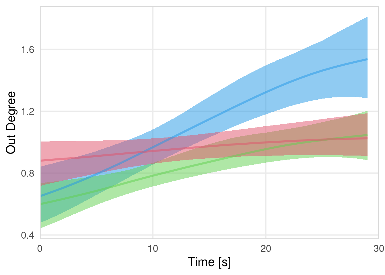
Out degree VP
m.events.s.OutDegree.VP.data  <- resource_discoveries_data_vp %>%
  filter(ResourceSpeed == 'slow', PlayerOrderCat == 'others') %>%
  filter(((Timepoint * 10) %% 10 == 0))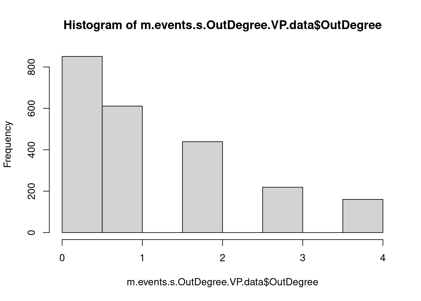
m.events.s.OutDegree.VP.formula <- brmsformula(
  OutDegree ~ gp(Timepoint, by = SignalingType),
  family = negbinomial()
  )
m.events.s.OutDegree.VP.priors <-
prior(normal(0, 1), class = "Intercept") +
prior(inv_gamma(10, 20), class = "lscale", coef = "gpTimepointSignalingTypeVP_NS") +
prior(inv_gamma(10, 20), class = "lscale", coef = "gpTimepointSignalingTypeVP_S") +
prior(normal(0, 0.25), class = "sdgp", lb = 0)Prior predictive checks
m.events.s.OutDegree.VP.fit_prior <- brm(
  formula = m.events.s.OutDegree.VP.formula,
  prior   = m.events.s.OutDegree.VP.priors,
  data    = m.events.s.OutDegree.VP.data,
  chains  = 4,
  cores   = 4,
  seed    = 42,
  iter    = 2000,
  file = paste0(fits_path, 'resource_discoveries_slow_out_degree_vp_prior.rds'),
  backend = "cmdstanr",
  threads = threading(100),
  control = list(adapt_delta = 0.95),
  save_pars = save_pars(all = TRUE),
  sample_prior = "only"
)plot(conditional_effects(m.events.s.OutDegree.VP.fit_prior, ndraws = 20, spaghetti = TRUE), points = F, ask = F)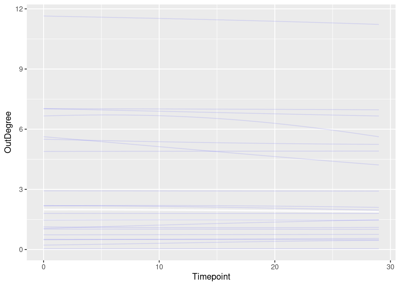
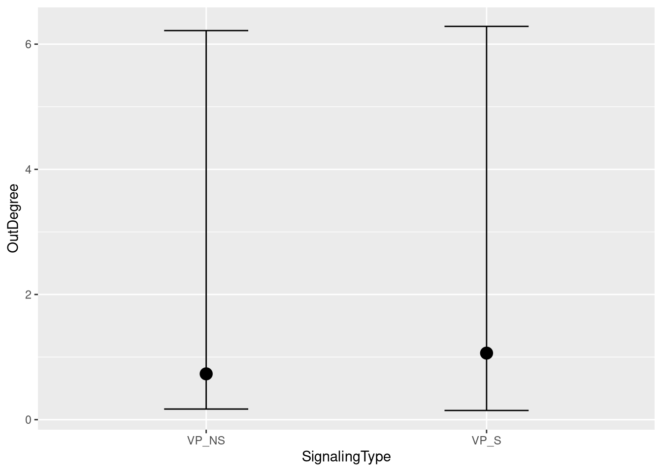
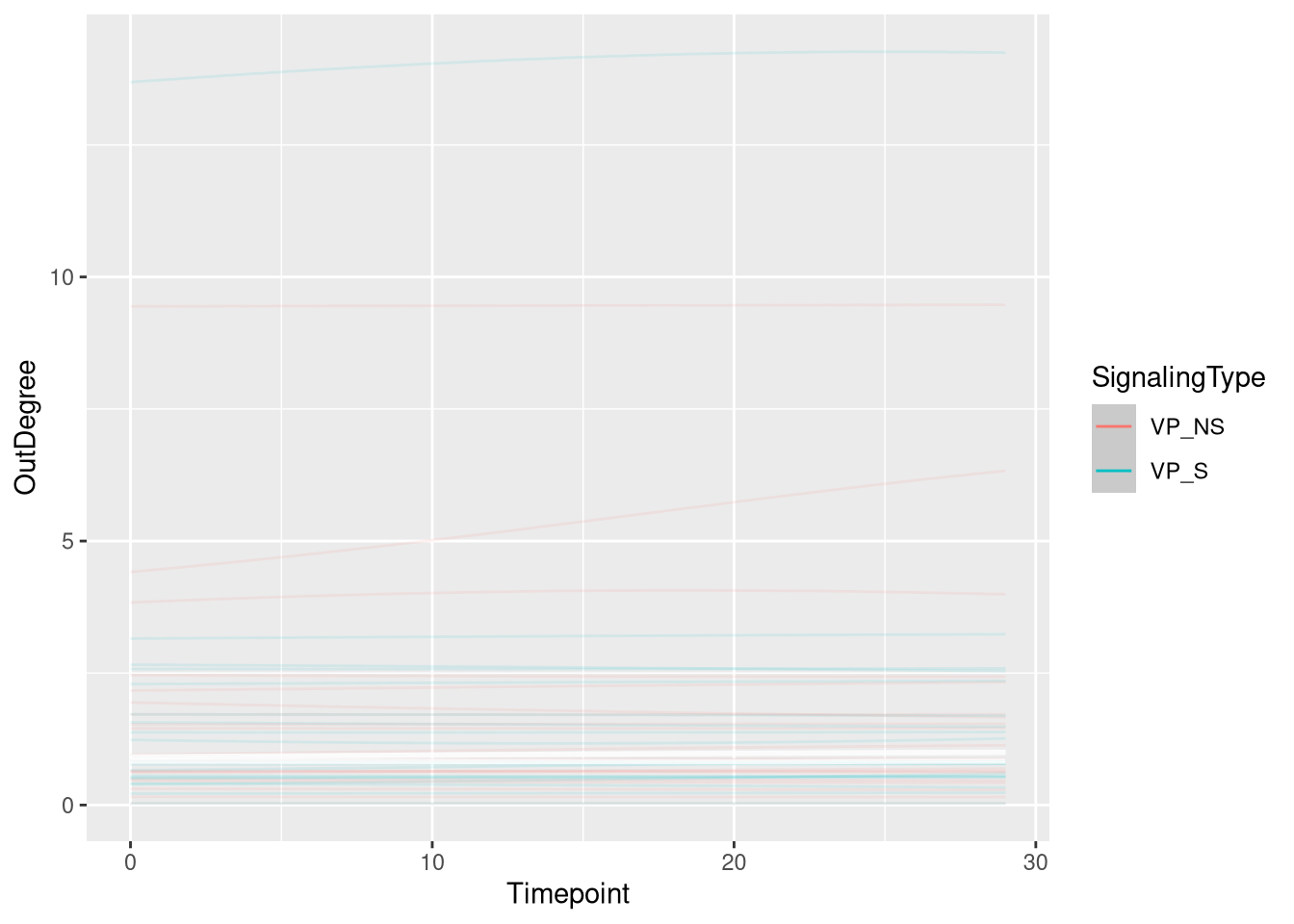
Model fitting
m.events.s.OutDegree.VP.fit <- brm(
  formula = m.events.s.OutDegree.VP.formula,
  prior   = m.events.s.OutDegree.VP.priors,
  data    = m.events.s.OutDegree.VP.data,
  chains = 4,
  cores = 4,
  seed = 42,
  warmup = 500,
  iter = 2000,
  file = paste0(fits_path, 'resource_discoveries_slow_out_degree_vp.rds'),
  backend = "cmdstanr",
  threads = threading(100),
  control = list(adapt_delta = 0.95),
  save_pars = save_pars(all = TRUE)
)## Family: negbinomial
## Links: mu = log; shape = identity
## Formula: OutDegree ~ gp(Timepoint, by = SignalingType)
## Data: m.events.s.OutDegree.VP.data (Number of observations: 2280)
## Draws: 4 chains, each with iter = 2000; warmup = 500; thin = 1;
## total post-warmup draws = 6000
##
## Gaussian Process Hyperparameters:
## Estimate Est.Error l-95% CI u-95% CI Rhat Bulk_ESS Tail_ESS
## sdgp(gpTimepointSignalingTypeVP_NS) 0.27 0.14 0.02 0.58 1.00 2349 1609
## sdgp(gpTimepointSignalingTypeVP_S) 0.44 0.13 0.23 0.72 1.00 4456 4018
## lscale(gpTimepointSignalingTypeVP_NS) 2.06 0.71 1.13 3.84 1.00 6021 3980
## lscale(gpTimepointSignalingTypeVP_S) 1.69 0.45 1.04 2.75 1.00 4739 4052
##
## Regression Coefficients:
## Estimate Est.Error l-95% CI u-95% CI Rhat Bulk_ESS Tail_ESS
## Intercept 0.16 0.21 -0.25 0.60 1.00 1606 2757
##
## Further Distributional Parameters:
## Estimate Est.Error l-95% CI u-95% CI Rhat Bulk_ESS Tail_ESS
## shape 4.28 0.69 3.17 5.86 1.00 8042 4021
##
## Draws were sampled using sample(hmc). For each parameter, Bulk_ESS
## and Tail_ESS are effective sample size measures, and Rhat is the potential
## scale reduction factor on split chains (at convergence, Rhat = 1).Model diagnostics
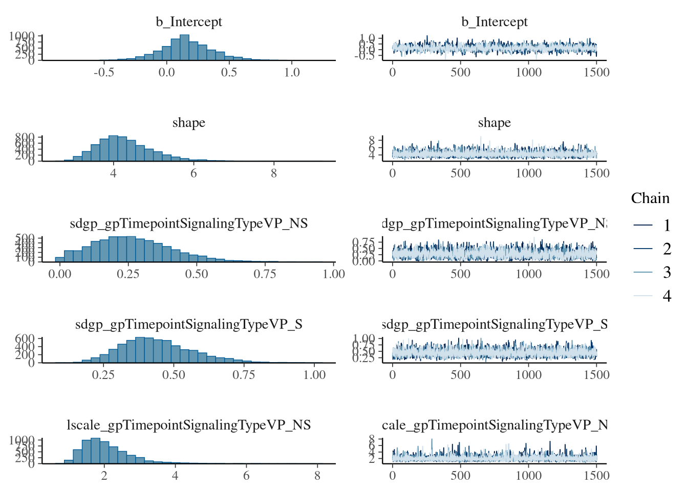
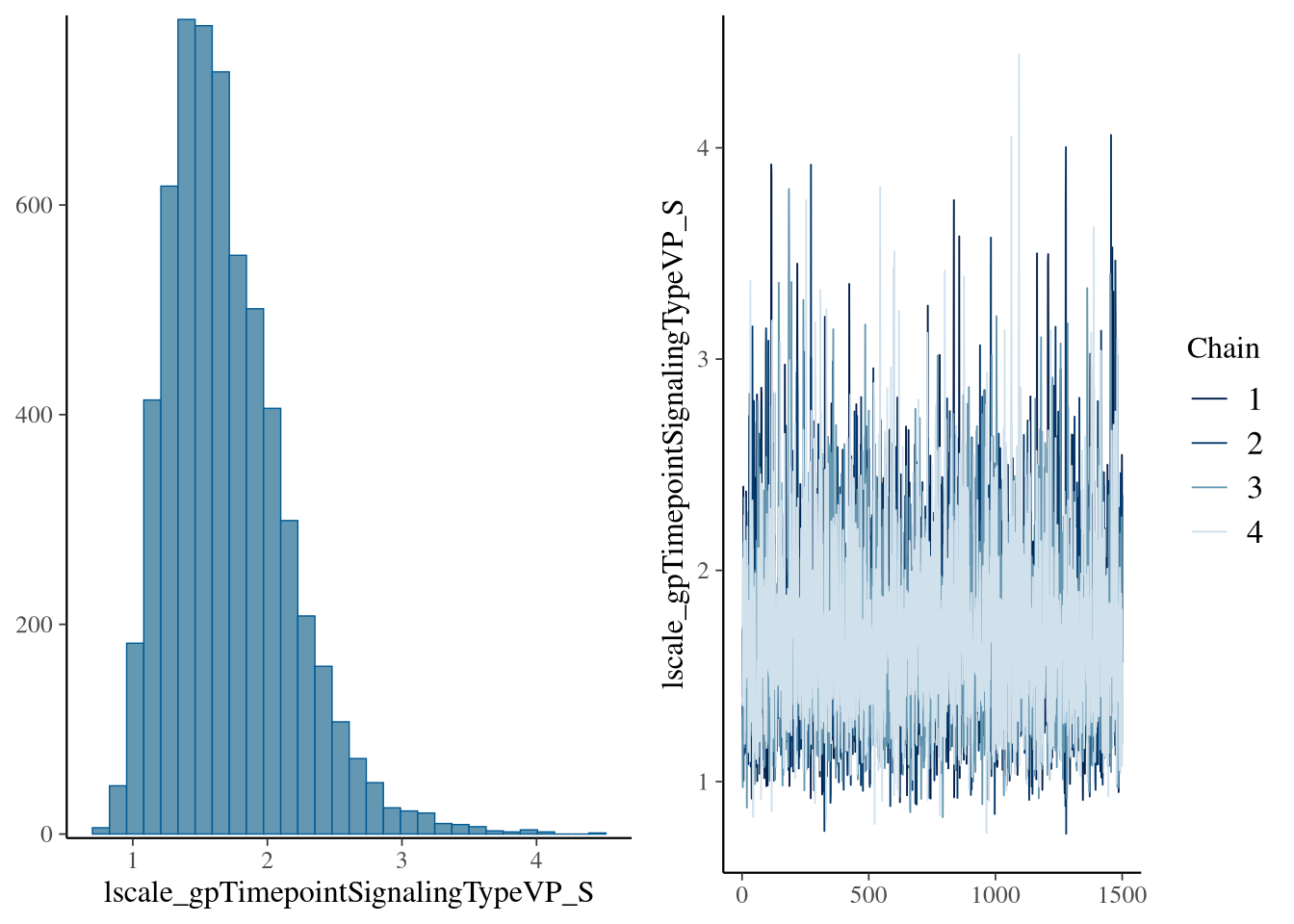
m.events.s.OutDegree.VP.me <- conditional_effects(m.events.s.OutDegree.VP.fit, ndraws = 200, spaghetti = TRUE)
plot(m.events.s.OutDegree.VP.me, ask = FALSE, points = F)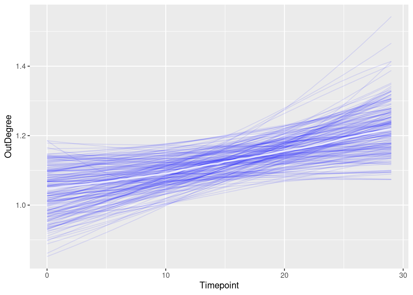
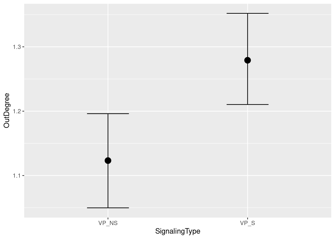
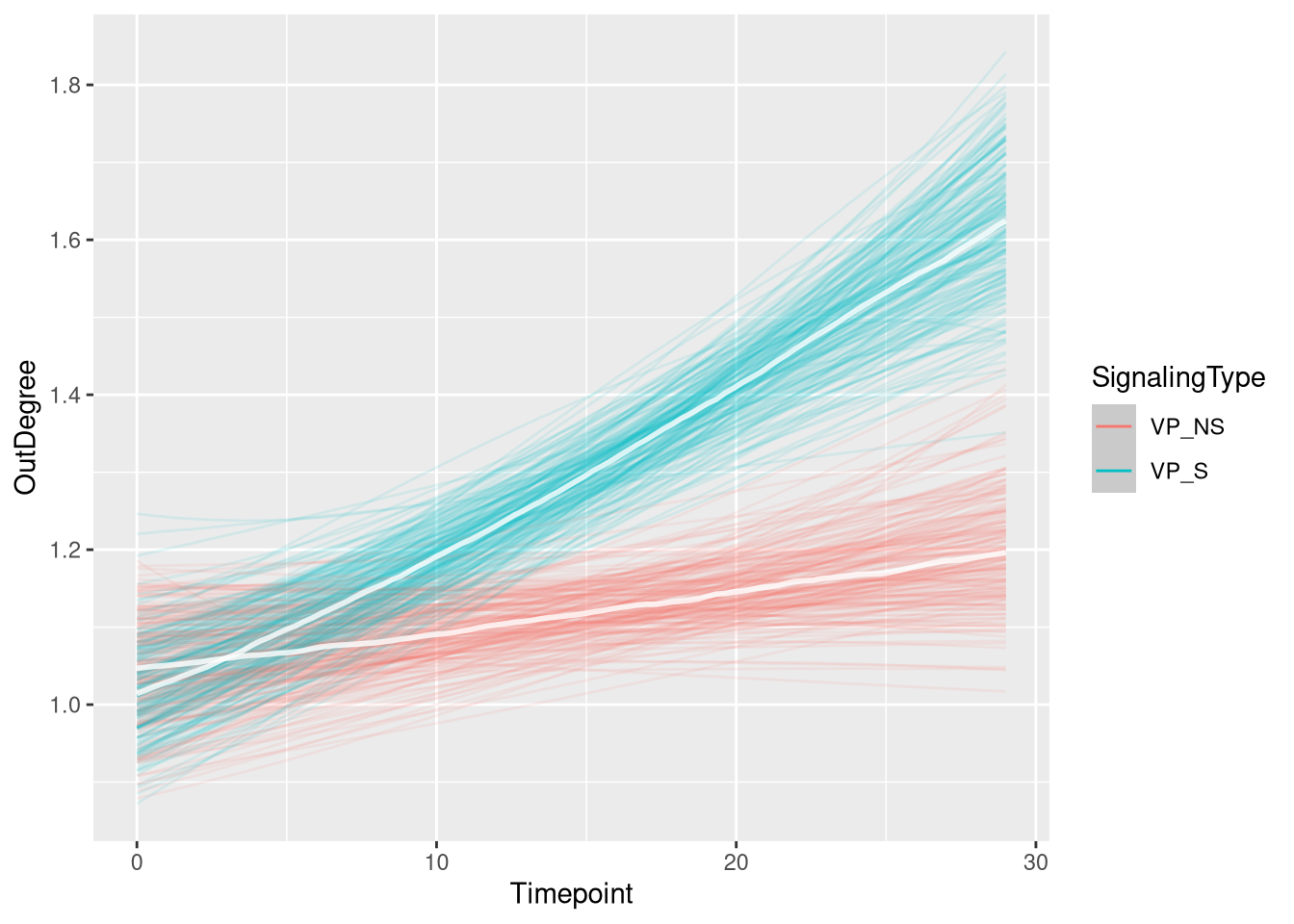
Figure
m.events.s.OutDegree.VP.draws <- m.events.s.OutDegree.VP.data  %>%
  mutate(SignalingType = factor(SignalingType, levels = c('VP_NS', 'VP_S'))) %>%
  data_grid(Timepoint, SignalingType) %>%
  tidybayes::add_epred_draws(m.events.s.OutDegree.VP.fit, allow_new_levels = TRUE,
                             re_formula = m.events.s.OutDegree.VP.formula)
events_slow_outdegree_vp_fig <- m.events.s.OutDegree.VP.draws %>%
ggplot(aes(x = Timepoint, y = .epred, fill = SignalingType, color = SignalingType)) +
stat_lineribbon(aes(group = paste(group, ...width..)), .width = c(.9), alpha = 1/2) +
theme_nice(legend.pos = 'none') +
scale_color_manual(breaks = c('VP_NS', 'VP_S'),
aesthetics = c("colour", "fill"),
values = c("#000000", "#DF536B"),
guide = guide_legend(
title = "Signaling",
)
) +
theme_clean() +
panel_border() +
theme(legend.position = "none") +
scale_x_continuous(
limits = c(0, 30),
expand = expansion(mult = c(0, 0))
) +
labs(x = "Time [s]",
y = "Out Degree")
events_slow_outdegree_vp_fig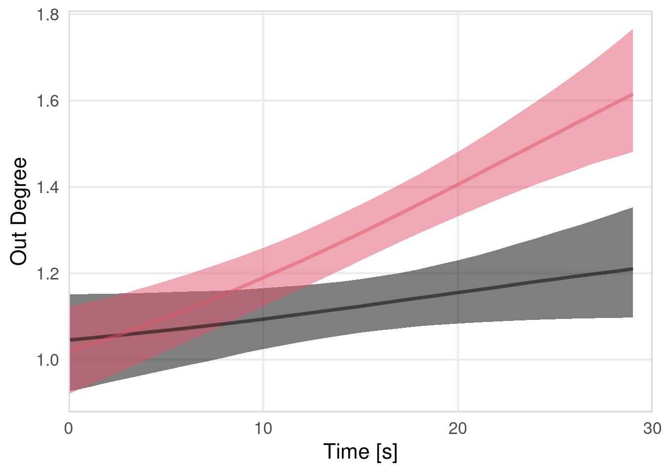
In degree
m.events.s.InDegree.data <- resource_discoveries_data %>%
  filter(ResourceSpeed == 'slow', SignalingType != 'A', PlayerOrderCat == 'first') %>%
  filter(((Timepoint * 10) %% 10 == 0))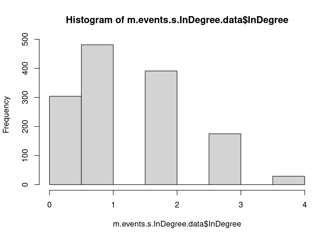
m.events.s.InDegree.formula <- brmsformula(
  InDegree ~ gp(Timepoint, by = SignalingType),
  family = poisson(link = "log")
  )
m.events.s.InDegree.priors <-
prior(normal(0, 1), class = "Intercept") +
prior(inv_gamma(10, 20), class = "lscale", coef = "gpTimepointSignalingTypeFP") +
prior(inv_gamma(10, 20), class = "lscale", coef = "gpTimepointSignalingTypeNP") +
prior(inv_gamma(10, 20), class = "lscale", coef = "gpTimepointSignalingTypeVP") +
prior(normal(0, 0.25), class = "sdgp", lb = 0)Prior predictive checks
m.events.s.InDegree.fit_prior <- brm(
  formula = m.events.s.InDegree.formula,
  prior   = m.events.s.InDegree.priors,
  data    = m.events.s.InDegree.data,
  chains  = 4,
  cores   = 4,
  seed    = 42,
  iter    = 2000,
  file = paste0(fits_path, 'resource_discoveries_slow_in_degree_prior.rds'),
  backend = "cmdstanr",
  threads = threading(100),
  control = list(adapt_delta = 0.95),
  save_pars = save_pars(all = TRUE),
  sample_prior = "only"
)plot(conditional_effects(m.events.s.InDegree.fit_prior, ndraws = 20, spaghetti = TRUE), points = F, ask = F)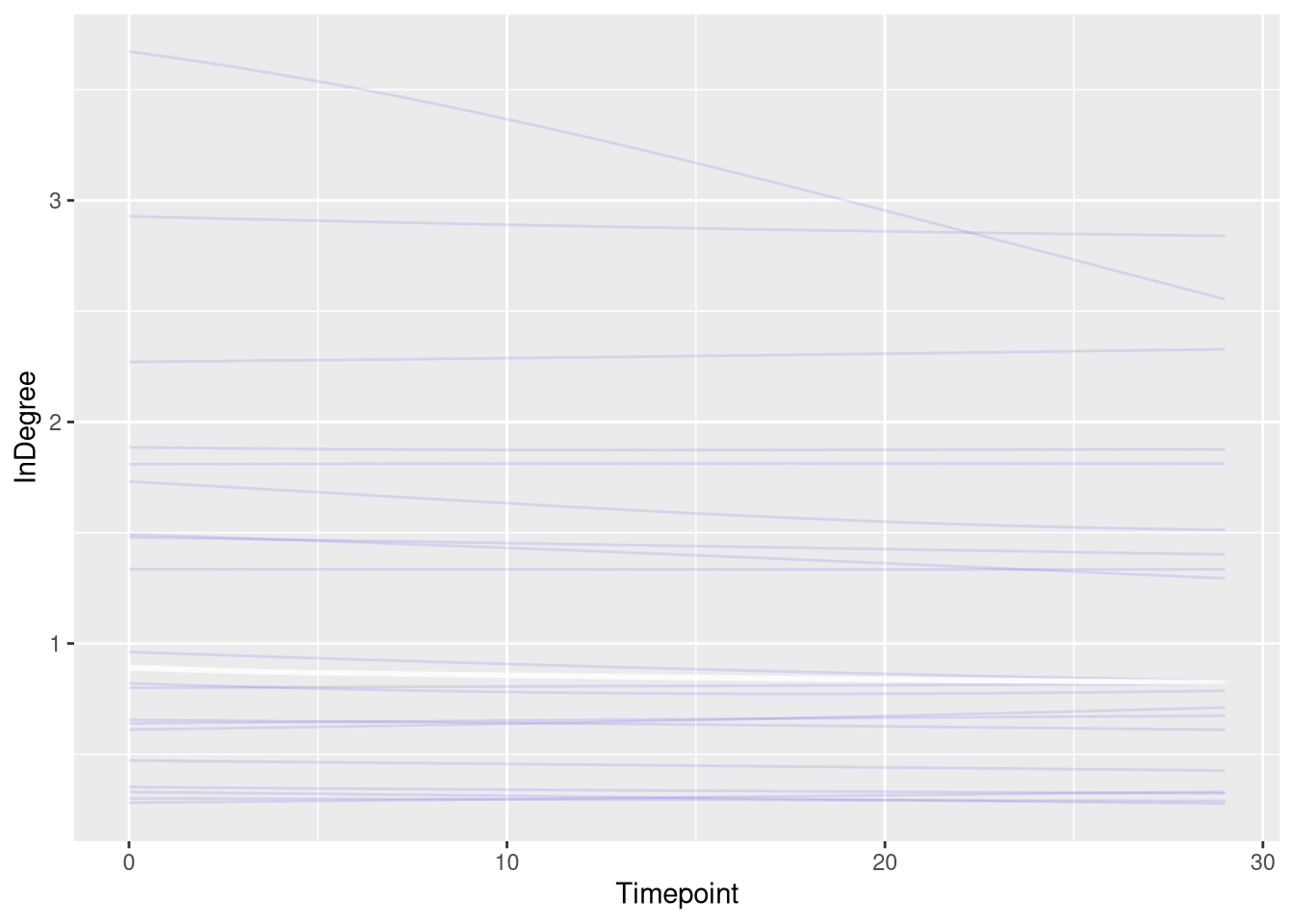
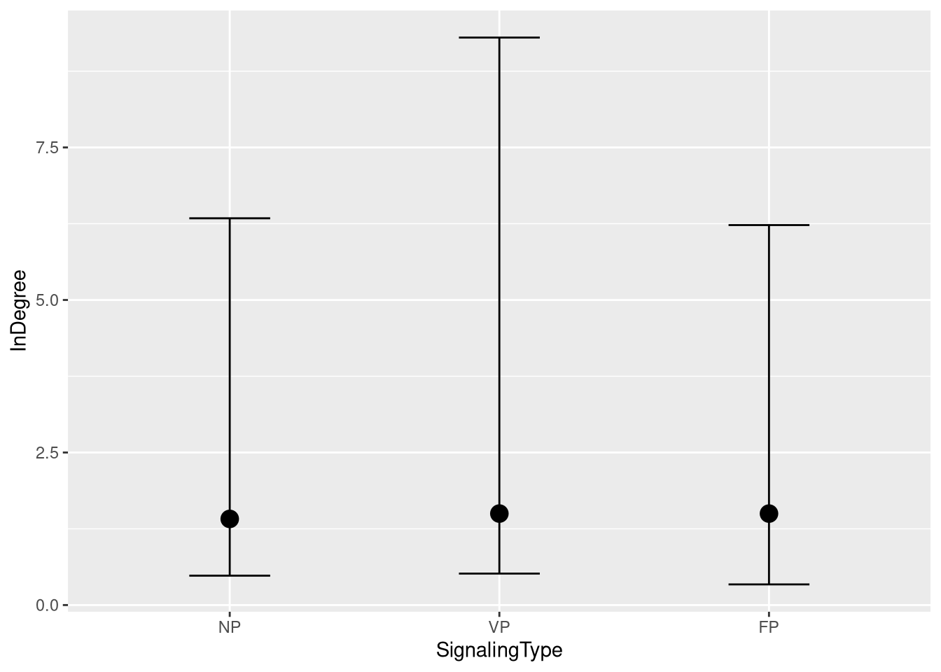
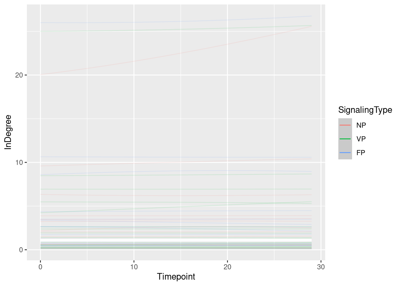
Model fitting
m.events.s.InDegree.fit <- brm(
  formula = m.events.s.InDegree.formula,
  prior   = m.events.s.InDegree.priors,
  data    = m.events.s.InDegree.data,
  chains = 4,
  cores = 4,
  seed = 42,
  warmup = 500,
  iter = 2000,
  file = paste0(fits_path, 'resource_discoveries_slow_in_degree.rds'),
  backend = "cmdstanr",
  threads = threading(100),
  control = list(adapt_delta = 0.95),
  save_pars = save_pars(all = TRUE)
)## Family: poisson
## Links: mu = log
## Formula: InDegree ~ gp(Timepoint, by = SignalingType)
## Data: m.events.s.InDegree.data (Number of observations: 1380)
## Draws: 4 chains, each with iter = 2000; warmup = 500; thin = 1;
## total post-warmup draws = 6000
##
## Gaussian Process Hyperparameters:
## Estimate Est.Error l-95% CI u-95% CI Rhat Bulk_ESS Tail_ESS
## sdgp(gpTimepointSignalingTypeNP) 0.17 0.13 0.01 0.48 1.00 3178 3350
## sdgp(gpTimepointSignalingTypeVP) 0.43 0.14 0.19 0.74 1.00 5898 3901
## sdgp(gpTimepointSignalingTypeFP) 0.37 0.15 0.11 0.69 1.00 4357 2722
## lscale(gpTimepointSignalingTypeNP) 2.21 0.78 1.17 4.20 1.00 12379 4165
## lscale(gpTimepointSignalingTypeVP) 1.66 0.45 0.98 2.74 1.00 9218 4335
## lscale(gpTimepointSignalingTypeFP) 1.84 0.57 1.05 3.18 1.00 8527 4160
##
## Regression Coefficients:
## Estimate Est.Error l-95% CI u-95% CI Rhat Bulk_ESS Tail_ESS
## Intercept 0.25 0.15 -0.05 0.57 1.00 2368 2693
##
## Draws were sampled using sample(hmc). For each parameter, Bulk_ESS
## and Tail_ESS are effective sample size measures, and Rhat is the potential
## scale reduction factor on split chains (at convergence, Rhat = 1).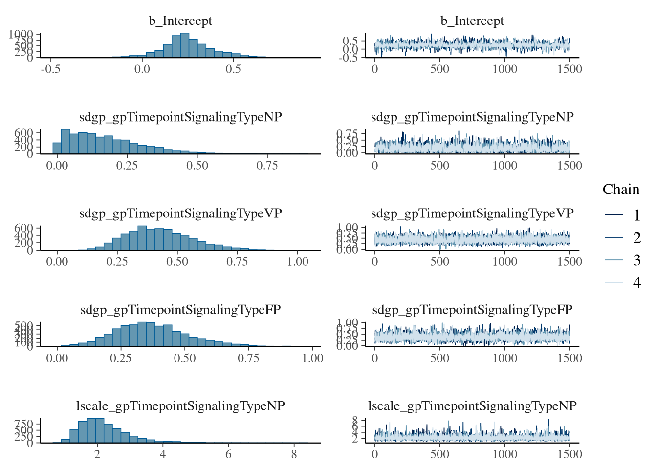
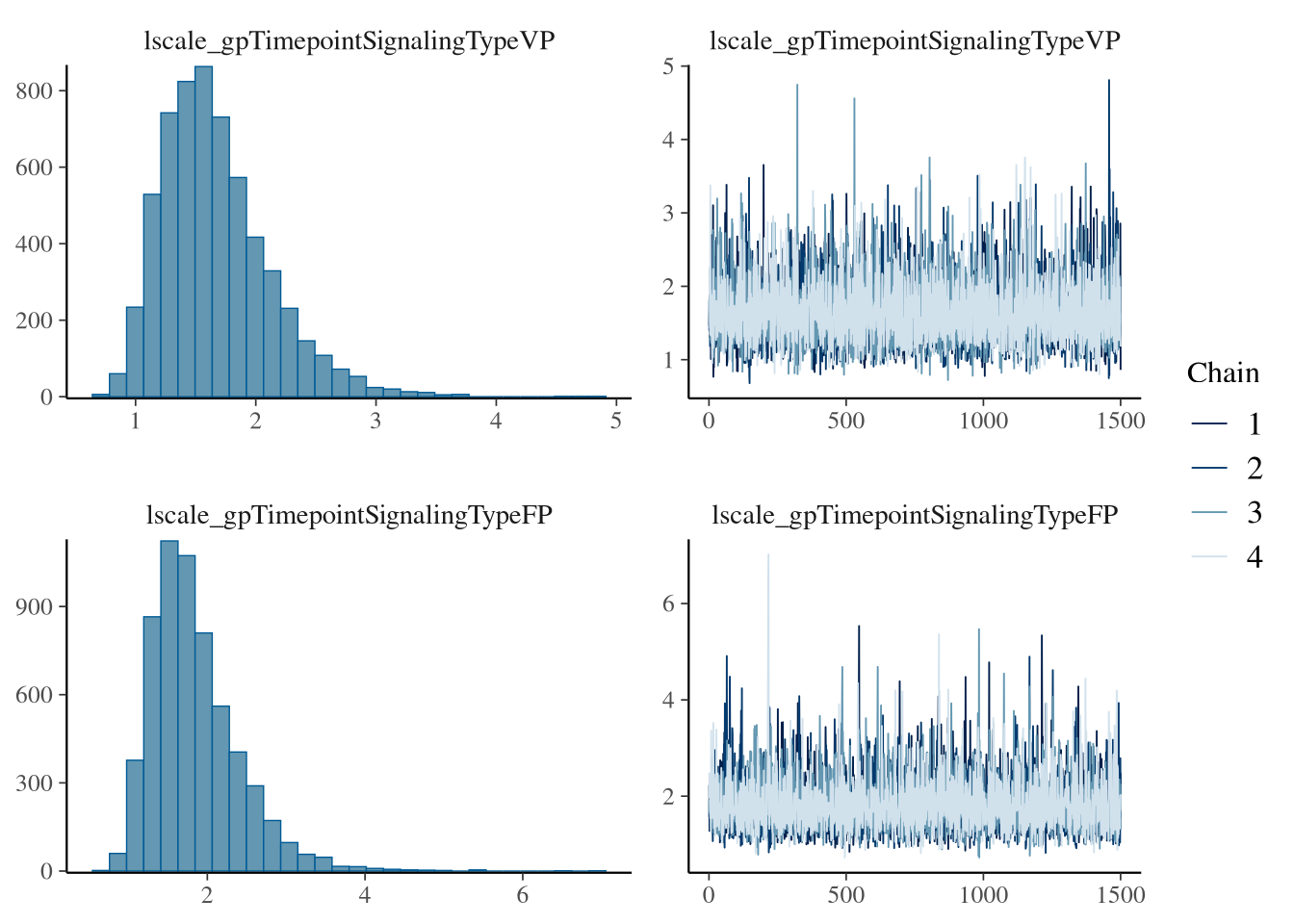
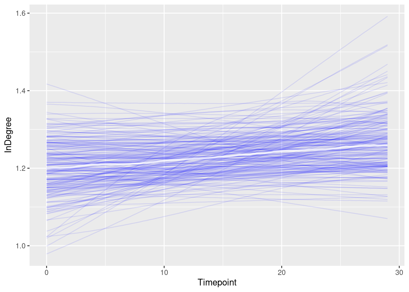
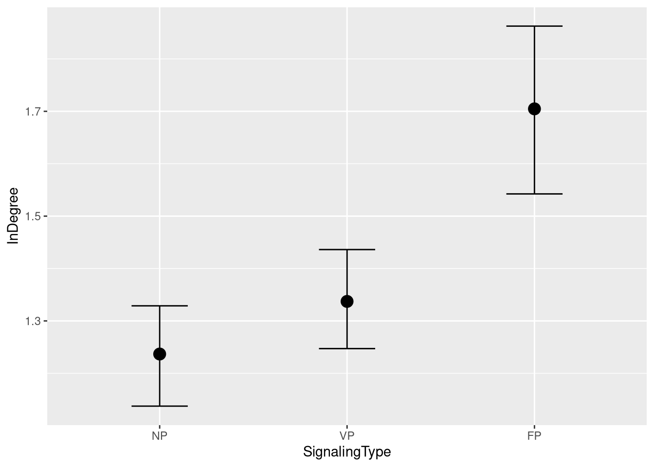
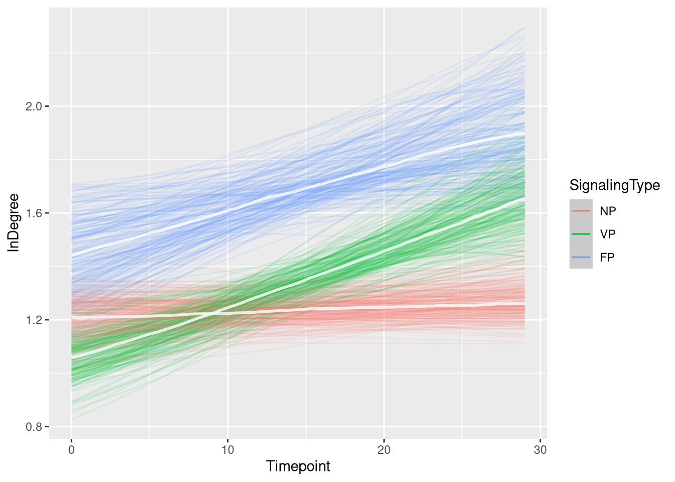
Figure
events_slow_in_degree_fig <- m.events.s.InDegree.draws %>%
  ggplot(aes(x = Timepoint, y = .epred, fill = SignalingType, color = SignalingType)) +
  stat_lineribbon(aes(group = paste(group, ...width..)), .width = c(.9), alpha = 1/2) +
  theme_nice(legend.pos = 'none') +
  scale_color_manual(breaks = c('NP', 'VP', 'FP'),
                     aesthetics = c("colour", "fill"),
                    values = c("#DF536B", "#61D04F", "#2297E6"),
                    guide = guide_legend(
                      title = "Signaling",
                     )
                    ) +
  theme_clean() +
  panel_border() +
  theme(legend.position    = "none") +
  scale_x_continuous(
    limits  = c(0, 30),
    expand  = expansion(mult = c(0, 0))
  ) +
  theme_clean() +
  panel_border() +
  theme(legend.position    = "none") +
  scale_x_continuous(
    limits  = c(0, 30),
    expand  = expansion(mult = c(0, 0))
  ) +
  labs(x = "Time [s]",
       y = "In Degree")


events_slow_in_degree_fig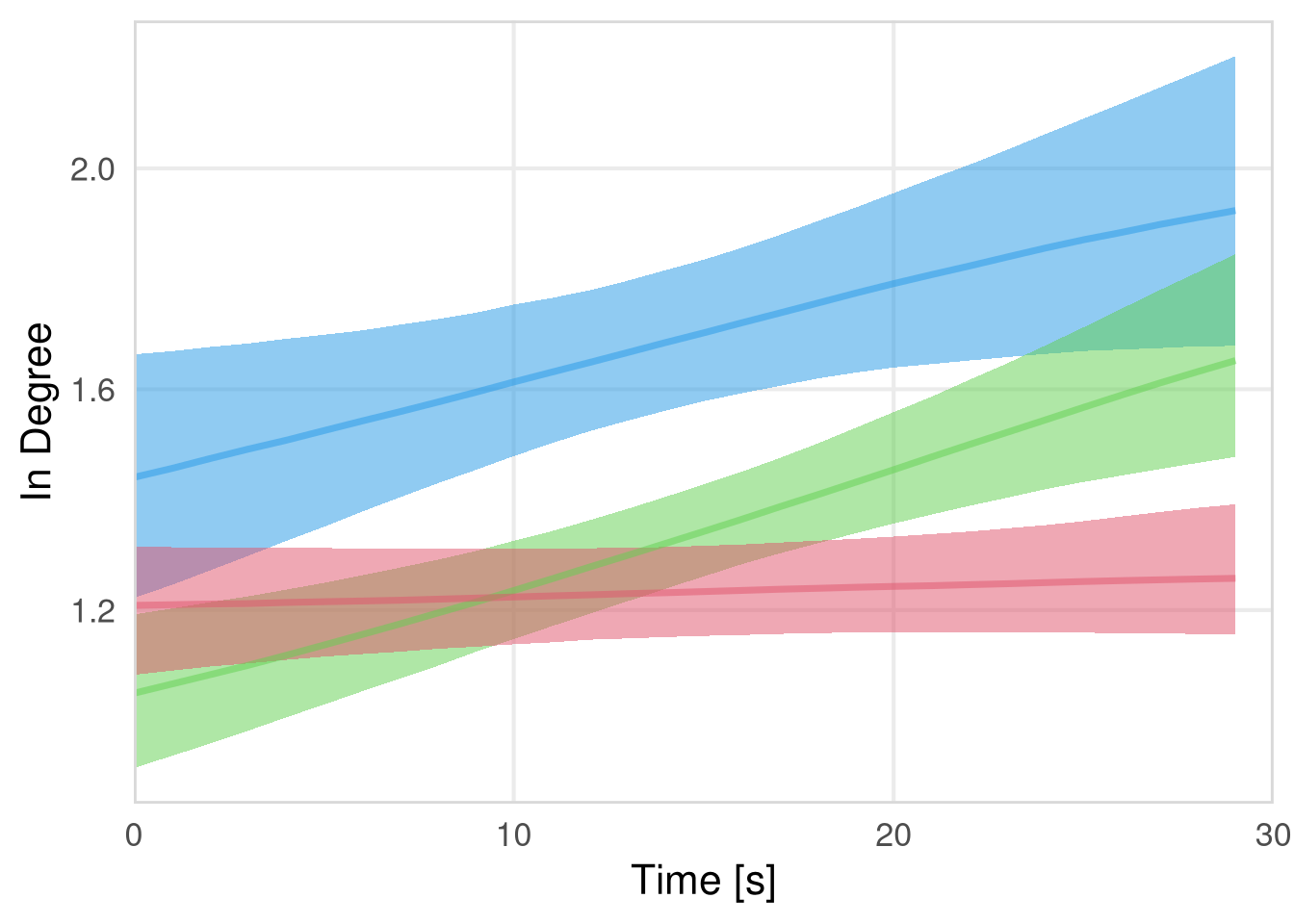
In degree (Others)
m.events.s.InDegree.Others.data <- resource_discoveries_data %>%
  filter(ResourceSpeed == 'slow', SignalingType != 'A', PlayerOrderCat == 'others') %>%
  filter(((Timepoint * 10) %% 10 == 0))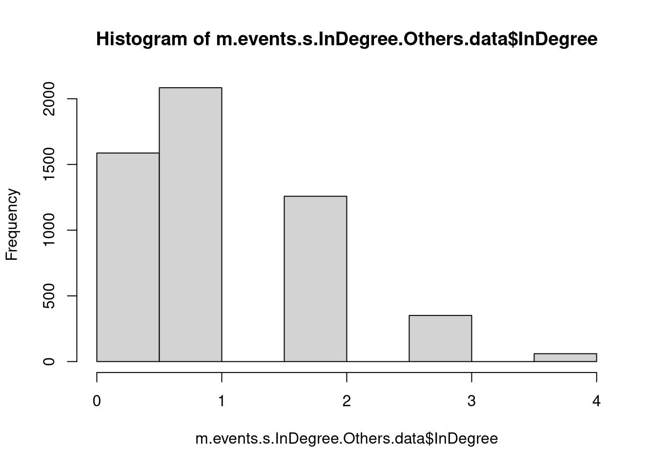
m.events.s.InDegree.Others.formula <- brmsformula(
  InDegree ~ gp(Timepoint, by = SignalingType),
  family = poisson(link = "log")
  )
m.events.s.InDegree.Others.priors <-
prior(normal(0, 1), class = "Intercept") +
prior(inv_gamma(10, 20), class = "lscale", coef = "gpTimepointSignalingTypeFP") +
prior(inv_gamma(10, 20), class = "lscale", coef = "gpTimepointSignalingTypeNP") +
prior(inv_gamma(10, 20), class = "lscale", coef = "gpTimepointSignalingTypeVP") +
prior(normal(0, 0.25), class = "sdgp", lb = 0)Prior predictive checks
m.events.s.InDegree.Others.fit_prior <- brm(
  formula = m.events.s.InDegree.Others.formula,
  prior   = m.events.s.InDegree.Others.priors,
  data    = m.events.s.InDegree.Others.data,
  chains  = 4,
  cores   = 4,
  seed    = 42,
  iter    = 2000,
  file = paste0(fits_path, 'resource_discoveries_slow_in_degree_others_prior.rds'),
  backend = "cmdstanr",
  threads = threading(100),
  control = list(adapt_delta = 0.95),
  save_pars = save_pars(all = TRUE),
  sample_prior = "only"
)plot(conditional_effects(m.events.s.InDegree.Others.fit_prior, ndraws = 20, spaghetti = TRUE), points = F, ask = F)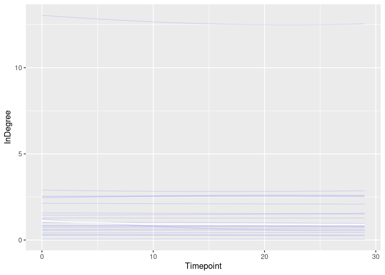
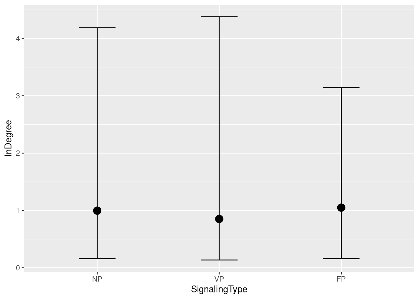
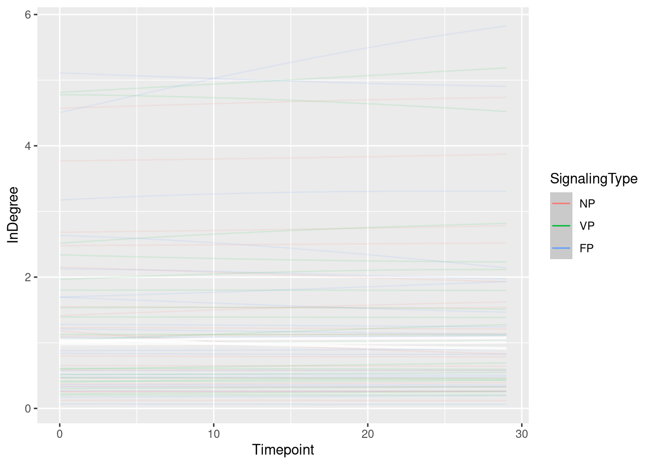
Model fitting
m.events.s.InDegree.Others.fit <- brm(
  formula = m.events.s.InDegree.Others.formula,
  prior   = m.events.s.InDegree.Others.priors,
  data    = m.events.s.InDegree.Others.data,
  chains = 4,
  cores = 4,
  seed = 42,
  warmup = 500,
  iter = 2000,
  file = paste0(fits_path, 'resource_discoveries_slow_in_degree_others.rds'),
  backend = "cmdstanr",
  threads = threading(100),
  control = list(adapt_delta = 0.95),
  save_pars = save_pars(all = TRUE)
)## Family: poisson
## Links: mu = log
## Formula: InDegree ~ gp(Timepoint, by = SignalingType)
## Data: m.events.s.InDegree.Others.data (Number of observations: 5340)
## Draws: 4 chains, each with iter = 2000; warmup = 500; thin = 1;
## total post-warmup draws = 6000
##
## Gaussian Process Hyperparameters:
## Estimate Est.Error l-95% CI u-95% CI Rhat Bulk_ESS Tail_ESS
## sdgp(gpTimepointSignalingTypeNP) 0.36 0.16 0.10 0.71 1.00 3273 2273
## sdgp(gpTimepointSignalingTypeVP) 0.42 0.13 0.21 0.71 1.00 7844 4582
## sdgp(gpTimepointSignalingTypeFP) 0.51 0.13 0.29 0.80 1.00 7103 4617
## lscale(gpTimepointSignalingTypeNP) 1.64 0.60 0.86 3.13 1.00 5783 4877
## lscale(gpTimepointSignalingTypeVP) 1.76 0.47 1.05 2.88 1.00 8974 4394
## lscale(gpTimepointSignalingTypeFP) 1.51 0.38 0.94 2.42 1.00 8765 4357
##
## Regression Coefficients:
## Estimate Est.Error l-95% CI u-95% CI Rhat Bulk_ESS Tail_ESS
## Intercept -0.07 0.21 -0.50 0.32 1.00 2818 3598
##
## Draws were sampled using sample(hmc). For each parameter, Bulk_ESS
## and Tail_ESS are effective sample size measures, and Rhat is the potential
## scale reduction factor on split chains (at convergence, Rhat = 1).Model diagnostics
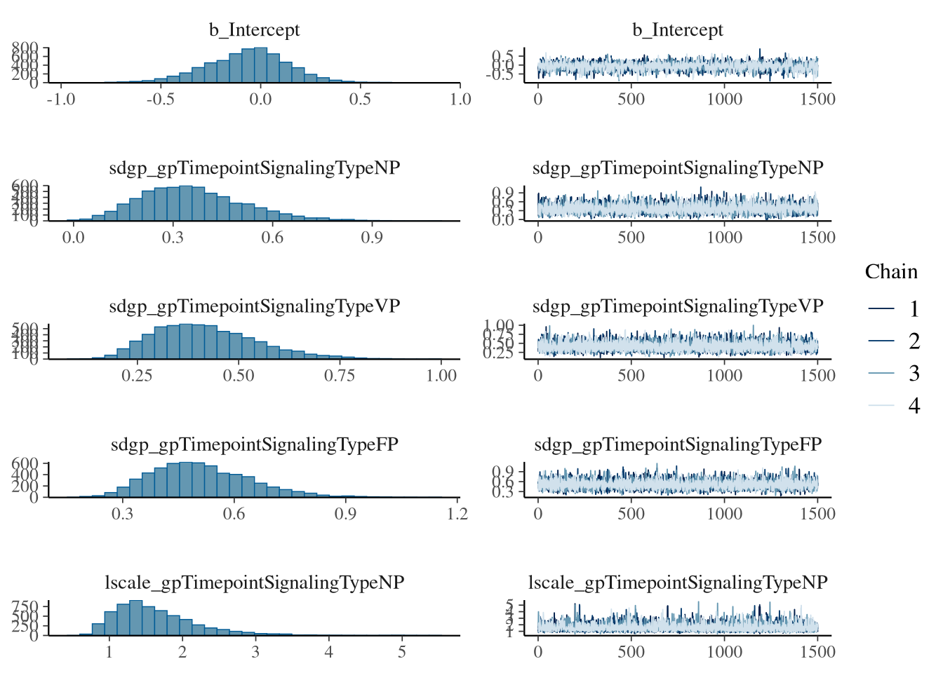
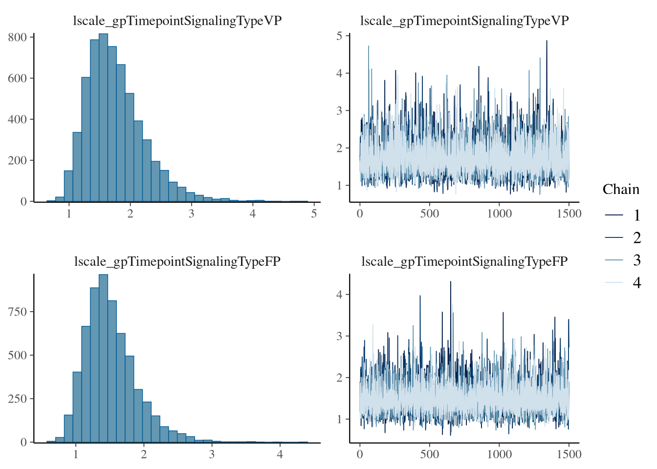
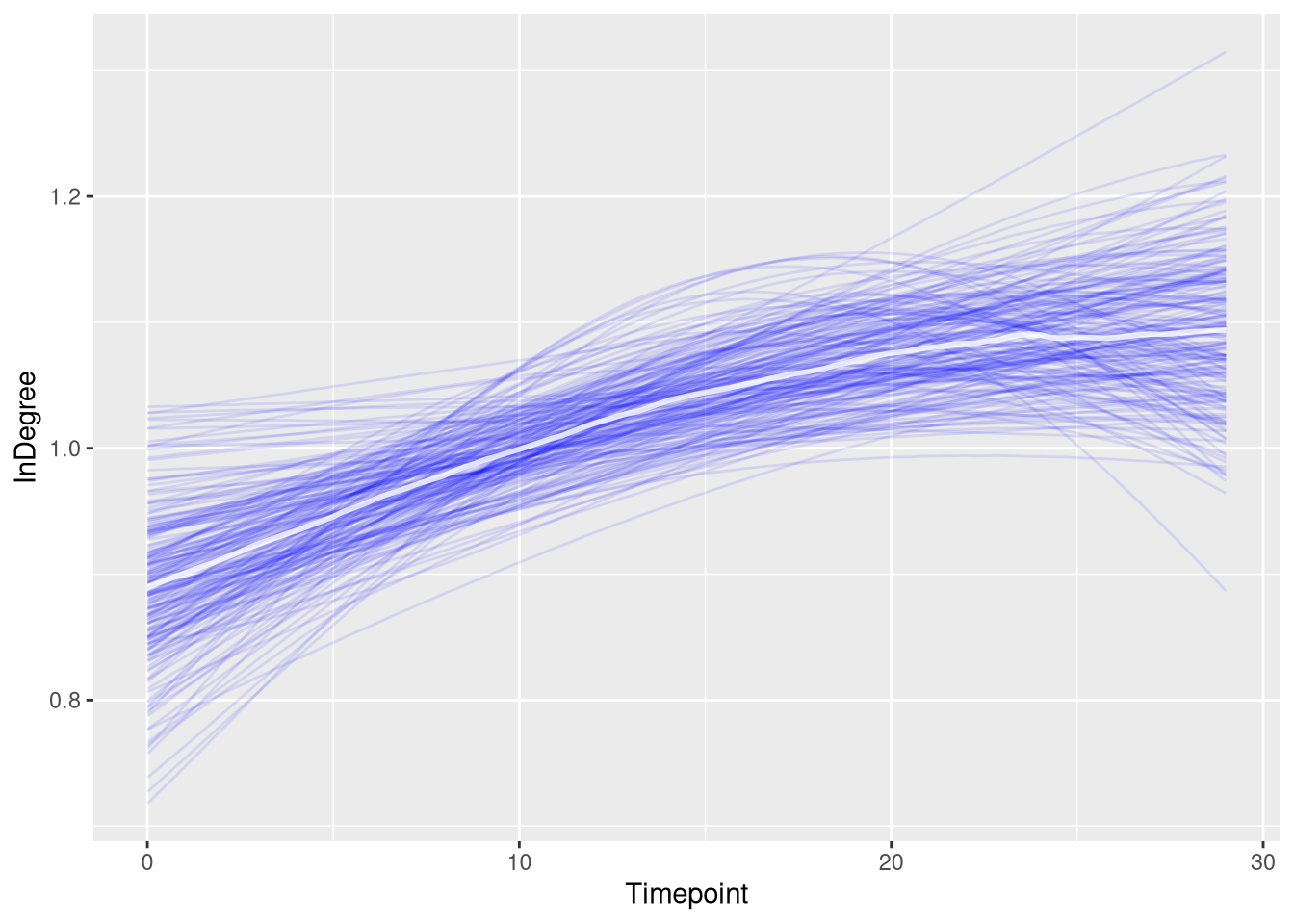
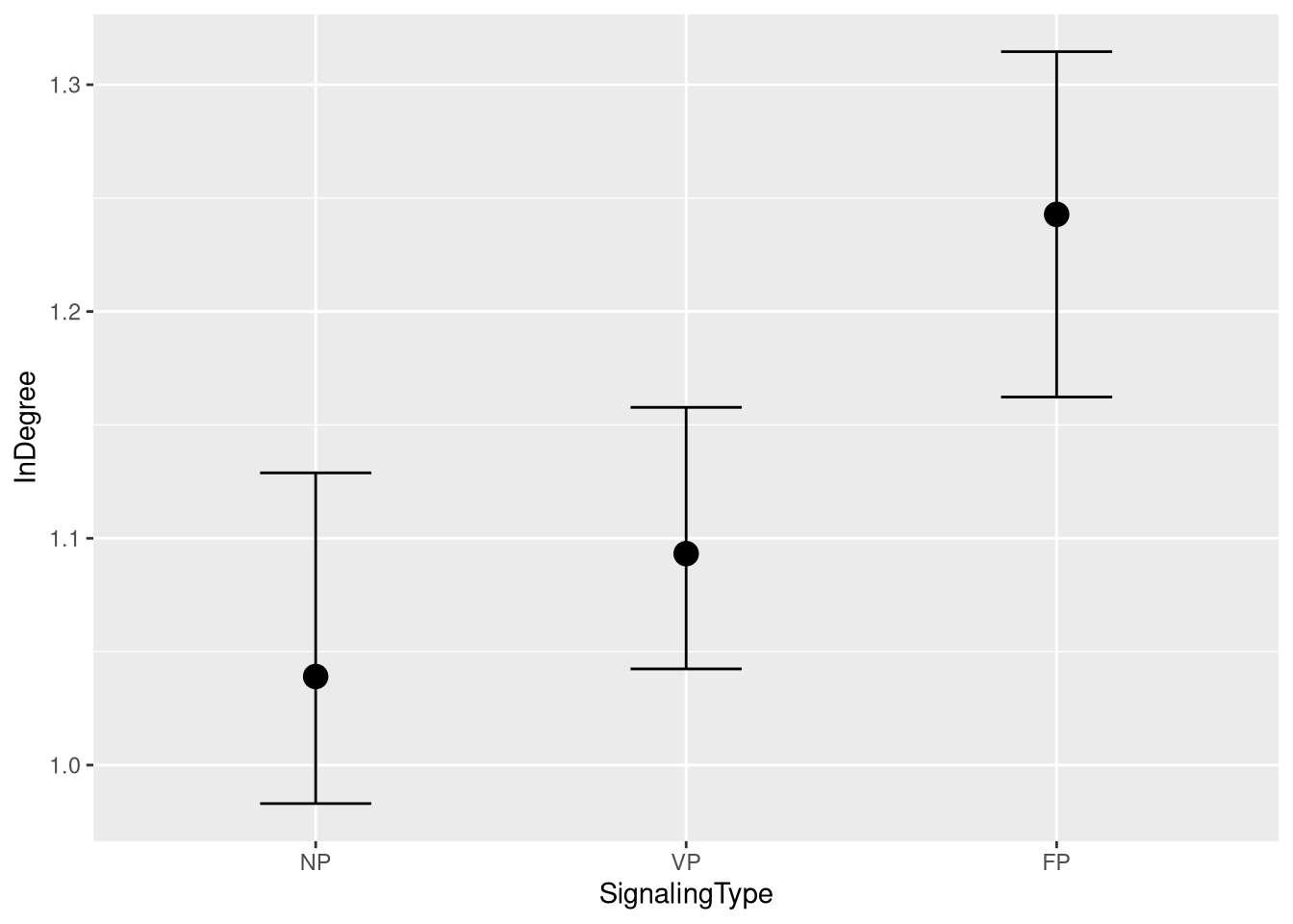
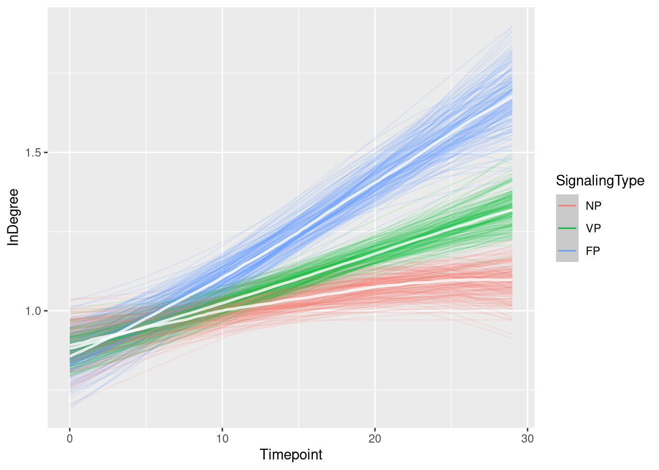
m.events.s.InDegree.Others.draws <- m.events.s.InDegree.Others.data %>%
  mutate(SignalingType = factor(SignalingType, levels = c('NP', 'VP', 'FP'))) %>%
  data_grid(Timepoint, SignalingType) %>%
  tidybayes::add_epred_draws(m.events.s.InDegree.Others.fit, allow_new_levels = TRUE,
                             re_formula = m.events.s.InDegree.Others.formula)
Figure
events_slow_in_degree_others_fig <- m.events.s.InDegree.Others.draws %>%
  ggplot(aes(x = Timepoint, y = .epred, fill = SignalingType, color = SignalingType)) +
  stat_lineribbon(aes(group = paste(group, ...width..)), .width = c(.9), alpha = 1/2) +
  theme_nice(legend.pos = 'none') +
  scale_color_manual(breaks = c('NP', 'VP', 'FP'),
                     aesthetics = c("colour", "fill"),
                    values = c("#DF536B", "#61D04F", "#2297E6"),
                    guide = guide_legend(
                      title = "Signaling",
                     )
                    ) +
  theme_clean() +
  panel_border() +
  theme(legend.position    = "none") +
  scale_x_continuous(
    limits  = c(0, 30),
    expand  = expansion(mult = c(0, 0))
  ) +
  theme_clean() +
  panel_border() +
  theme(legend.position    = "none") +
  scale_x_continuous(
    limits  = c(0, 30),
    expand  = expansion(mult = c(0, 0))
  ) +
  labs(x = "Time [s]",
       y = "In Degree")


events_slow_in_degree_others_fig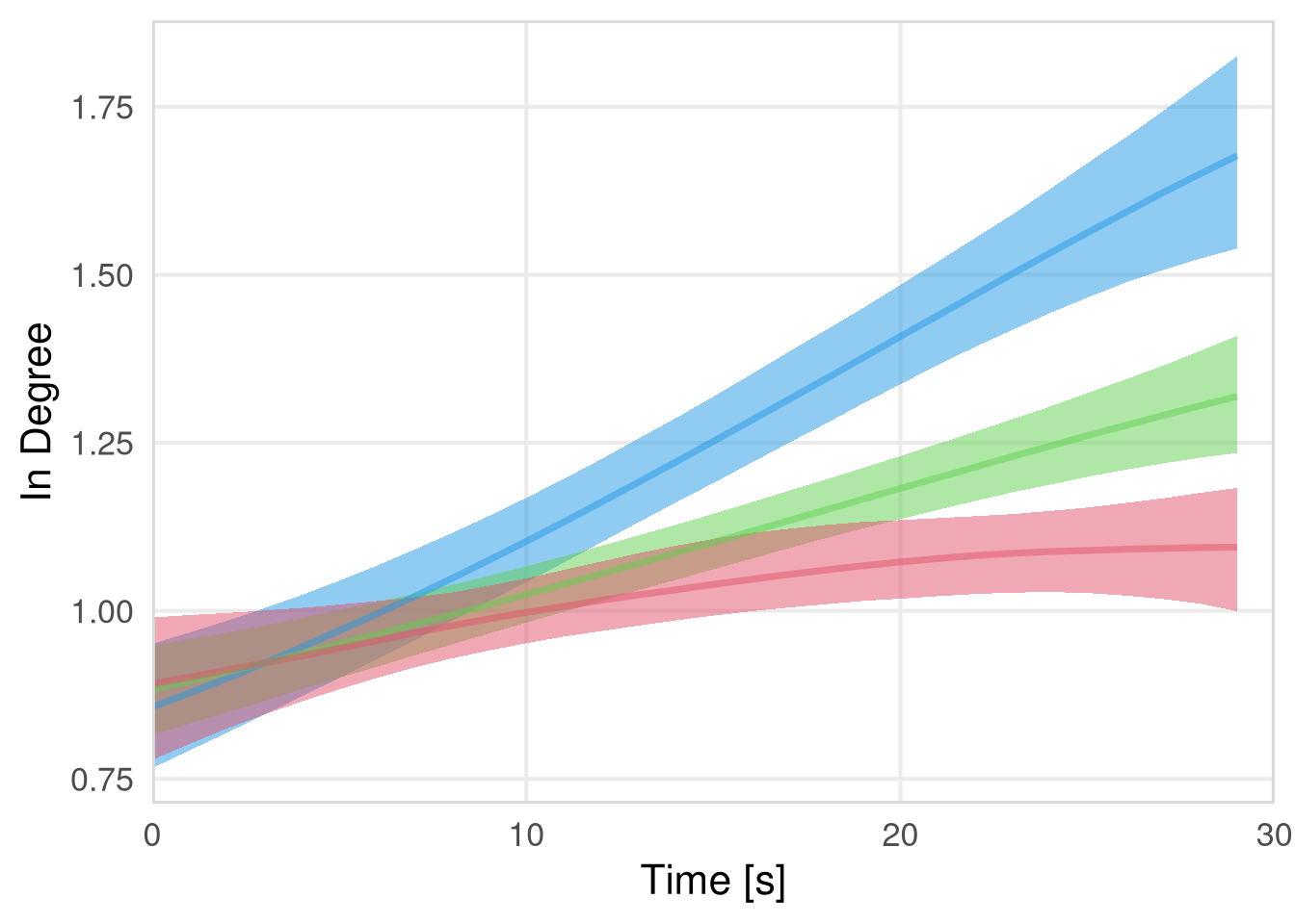
In degree VP
m.events.s.InDegree.VP.data <- resource_discoveries_data_vp %>%
  filter(ResourceSpeed == 'slow', PlayerOrderCat == 'first') %>%
  filter(((Timepoint * 10) %% 10 == 0))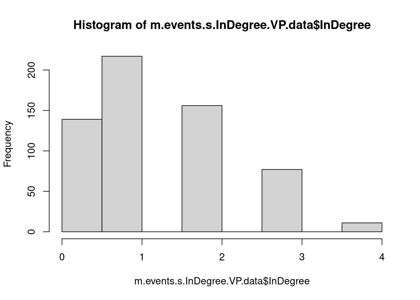
m.events.s.InDegree.VP.formula <- brmsformula(
  InDegree ~ gp(Timepoint, by = SignalingType),
  family = negbinomial()
  )
m.events.s.InDegree.VP.priors <-
prior(normal(0, 1), class = "Intercept") +
prior(inv_gamma(10, 20), class = "lscale", coef = "gpTimepointSignalingTypeVP_NS") +
prior(inv_gamma(10, 20), class = "lscale", coef = "gpTimepointSignalingTypeVP_S") +
prior(normal(0, 0.1), class = "sdgp", lb = 0)Prior predictive checks
m.events.s.InDegree.VP.fit_prior <- brm(
  formula = m.events.s.InDegree.VP.formula,
  prior   = m.events.s.InDegree.VP.priors,
  data    = m.events.s.InDegree.VP.data,
  chains  = 4,
  cores   = 4,
  seed    = 42,
  iter    = 2000,
  file = paste0(fits_path, 'resource_discoveries_slow_in_degree_vp_prior.rds'),
  backend = "cmdstanr",
  threads = threading(100),
  control = list(adapt_delta = 0.95),
  save_pars = save_pars(all = TRUE),
  sample_prior = "only"
)plot(conditional_effects(m.events.s.InDegree.VP.fit_prior, ndraws = 20, spaghetti = TRUE), points = F, ask = F)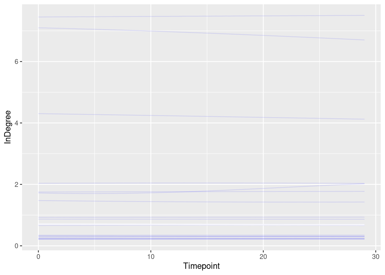
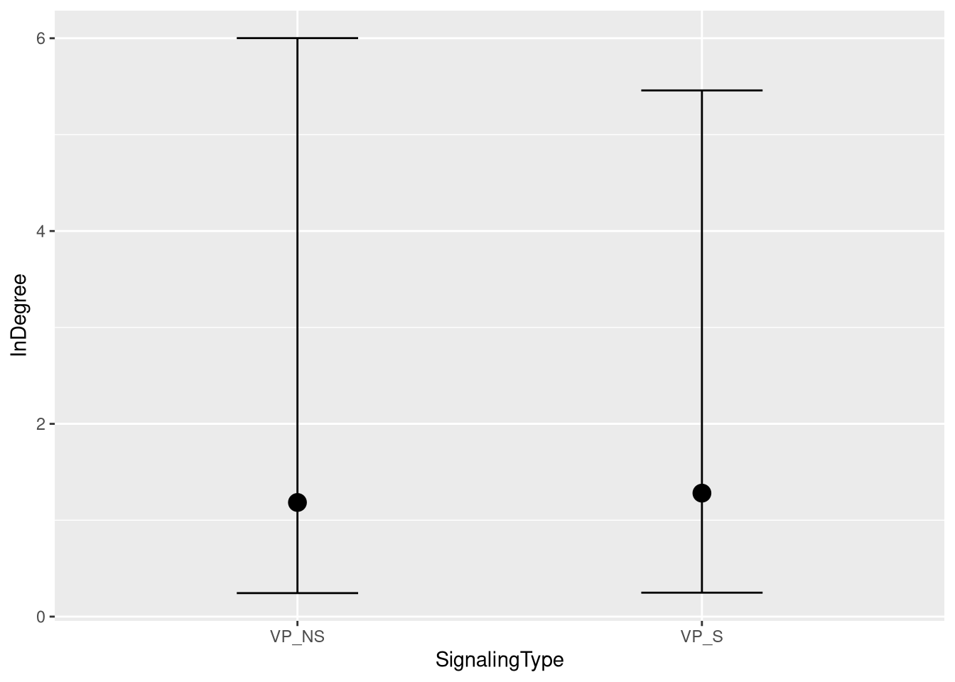
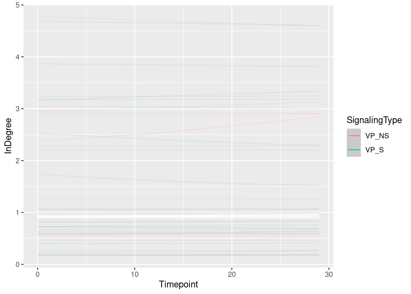
##  Family: negbinomial
##   Links: mu = log; shape = identity
## Formula: InDegree ~ gp(Timepoint, by = SignalingType)
##    Data: m.events.s.InDegree.VP.data (Number of observations: 600)
##   Draws: 4 chains, each with iter = 2000; warmup = 1000; thin = 1;
##          total post-warmup draws = 4000
##
## Gaussian Process Hyperparameters:
##                                       Estimate Est.Error l-95% CI u-95% CI Rhat Bulk_ESS Tail_ESS
## sdgp(gpTimepointSignalingTypeVP_NS)       0.08      0.06     0.00     0.22 1.00     3635     1707
## sdgp(gpTimepointSignalingTypeVP_S)        0.08      0.06     0.00     0.22 1.00     3614     1899
## lscale(gpTimepointSignalingTypeVP_NS)     2.23      0.80     1.14     4.27 1.00     5093     2773
## lscale(gpTimepointSignalingTypeVP_S)      2.24      0.82     1.15     4.34 1.00     5575     2501
##
## Regression Coefficients:
##           Estimate Est.Error l-95% CI u-95% CI Rhat Bulk_ESS Tail_ESS
## Intercept     0.01      0.99    -1.93     1.91 1.00     5944     2882
##
## Further Distributional Parameters:
##         Estimate    Est.Error l-95% CI u-95% CI Rhat Bulk_ESS Tail_ESS
## shape 3114684.60 195245161.46     0.13  4205.25 1.00     3644     1972
##
## Draws were sampled using sample(hmc). For each parameter, Bulk_ESS
## and Tail_ESS are effective sample size measures, and Rhat is the potential
## scale reduction factor on split chains (at convergence, Rhat = 1).
Model fitting
m.events.s.InDegree.VP.fit <- brm(
  formula = m.events.s.InDegree.VP.formula,
  prior   = m.events.s.InDegree.VP.priors,
  data    = m.events.s.InDegree.VP.data,
  chains = 4,
  cores = 4,
  seed = 42,
  warmup = 500,
  iter = 2000,
  file = paste0(fits_path, 'resource_discoveries_slow_in_degree_vp.rds'),
  backend = "cmdstanr",
  threads = threading(100),
  control = list(adapt_delta = 0.95),
  save_pars = save_pars(all = TRUE)
)## Family: negbinomial
## Links: mu = log; shape = identity
## Formula: InDegree ~ gp(Timepoint, by = SignalingType)
## Data: m.events.s.InDegree.VP.data (Number of observations: 600)
## Draws: 4 chains, each with iter = 2000; warmup = 500; thin = 1;
## total post-warmup draws = 6000
##
## Gaussian Process Hyperparameters:
## Estimate Est.Error l-95% CI u-95% CI Rhat Bulk_ESS Tail_ESS
## sdgp(gpTimepointSignalingTypeVP_NS) 0.08 0.06 0.00 0.23 1.00 2900 2835
## sdgp(gpTimepointSignalingTypeVP_S) 0.24 0.07 0.10 0.38 1.00 1678 788
## lscale(gpTimepointSignalingTypeVP_NS) 2.20 0.79 1.15 4.09 1.00 11183 4585
## lscale(gpTimepointSignalingTypeVP_S) 1.43 0.47 0.84 2.53 1.00 4399 2762
##
## Regression Coefficients:
## Estimate Est.Error l-95% CI u-95% CI Rhat Bulk_ESS Tail_ESS
## Intercept 0.14 0.11 -0.05 0.39 1.00 2208 1050
##
## Further Distributional Parameters:
## Estimate Est.Error l-95% CI u-95% CI Rhat Bulk_ESS Tail_ESS
## shape 72729234.35 2607147261.58 51.04 2764955.50 1.00 4713 2708
##
## Draws were sampled using sample(hmc). For each parameter, Bulk_ESS
## and Tail_ESS are effective sample size measures, and Rhat is the potential
## scale reduction factor on split chains (at convergence, Rhat = 1).Model diagnostics
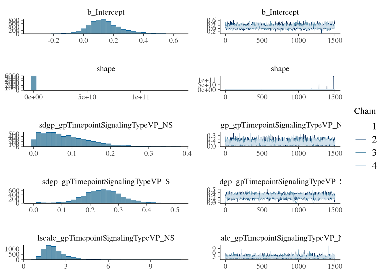
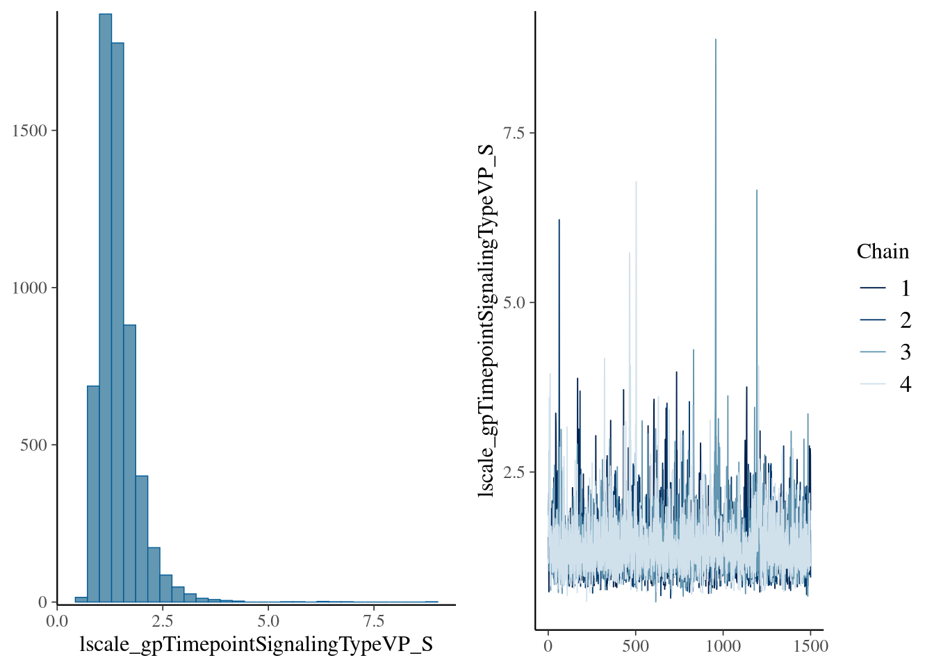
m.events.s.InDegree.VP.me <- conditional_effects(m.events.s.InDegree.VP.fit, ndraws = 200, spaghetti = TRUE)
plot(m.events.s.InDegree.VP.me, ask = FALSE, points = F)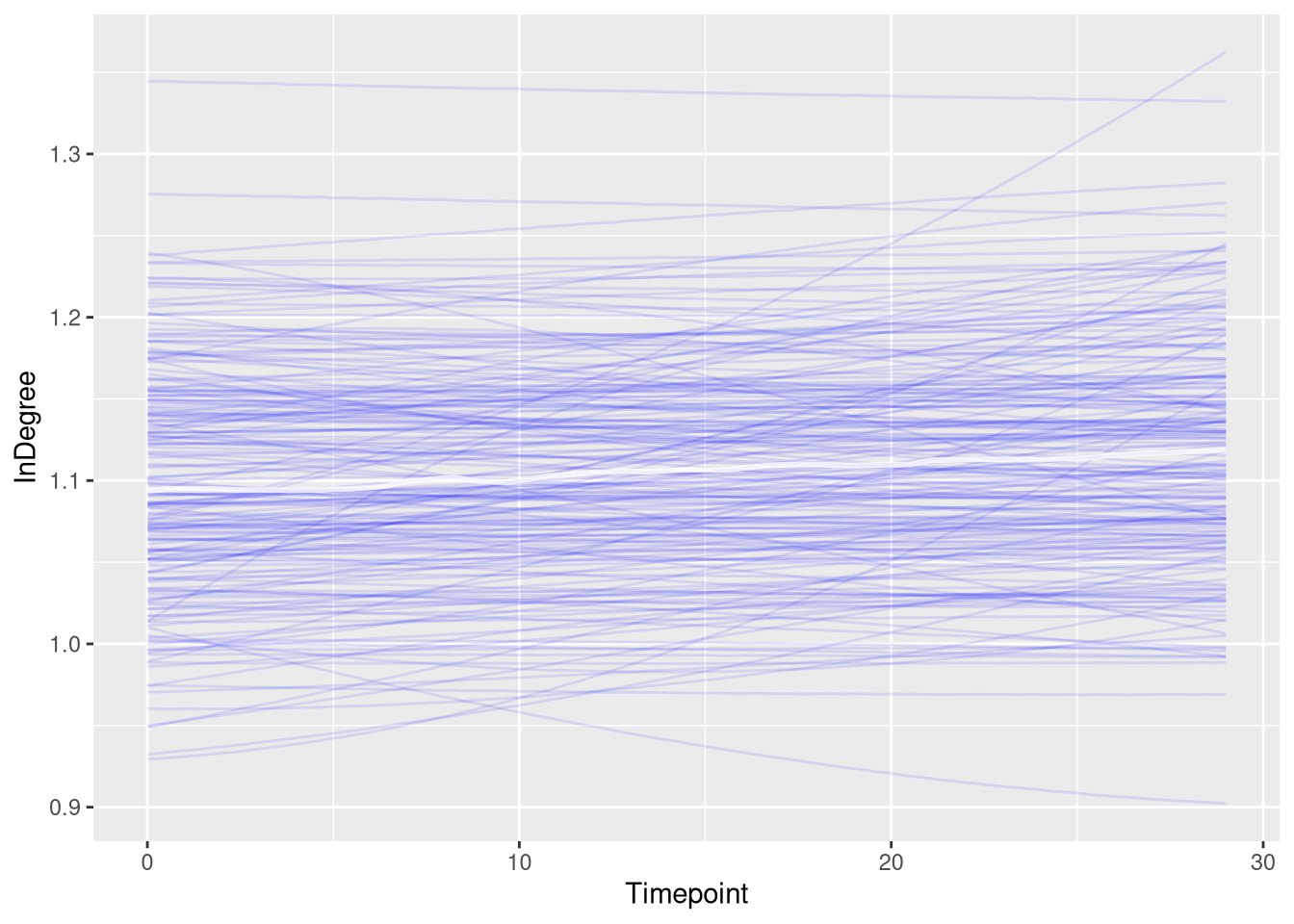
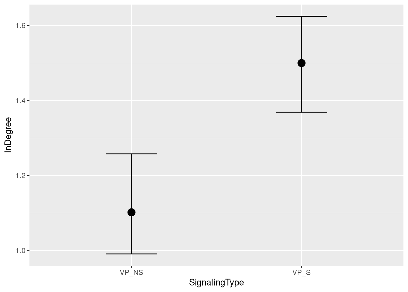
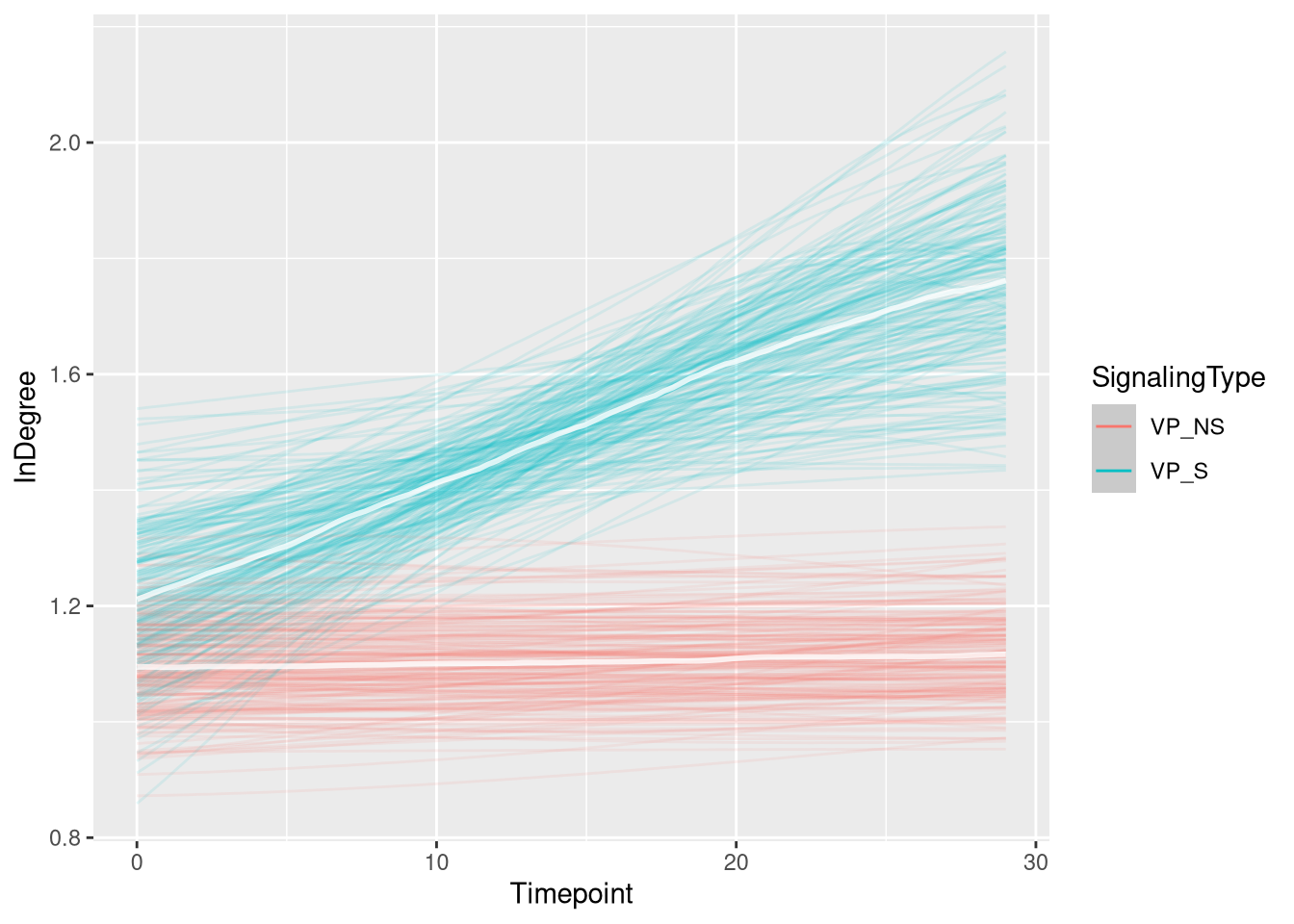
Figure
m.events.s.InDegree.VP.draws <- m.events.s.InDegree.VP.data %>%
  mutate(SignalingType = factor(SignalingType, levels = c('VP_NS', 'VP_S'))) %>%
  data_grid(Timepoint, SignalingType) %>%
  tidybayes::add_epred_draws(m.events.s.InDegree.VP.fit, allow_new_levels = TRUE, re_formula = m.events.s.InDegree.VP.formula)
events_slow_in_degree_vp_fig <- m.events.s.InDegree.VP.draws %>%
ggplot(aes(x = Timepoint, y = .epred, fill = SignalingType, color = SignalingType)) +
stat_lineribbon(aes(group = paste(group, ...width..)), .width = c(.9), alpha = 1/2) +
theme_nice(legend.pos = 'none') +
scale_color_manual(breaks = c('VP_NS', 'VP_S'),
aesthetics = c("colour", "fill"),
values = c("#000000", "#DF536B"),
guide = guide_legend(
title = "Signaling",
)
) +
theme_clean() +
panel_border() +
theme(legend.position = "none") +
scale_x_continuous(
limits = c(0, 30),
expand = expansion(mult = c(0, 0))
) +
labs(x = "Time [s]",
y = "In Degree")
events_slow_in_degree_vp_fig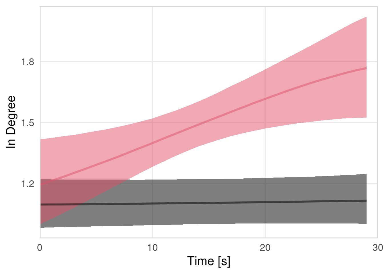
Combine plot
resource_discoveries_figure_slow <- ggarrange(
  ggarrange(events_slow_p_stay_fig, events_slow_in_degree_fig, nrow = 2, labels = c("", "")),
  ggarrange(events_slow_p_reach_fig, events_slow_outdegree_fig, nrow = 2, labels = c("", "")),
  ncol = 2,
  widths = c(1, 1)
)

resource_discoveries_figure_slow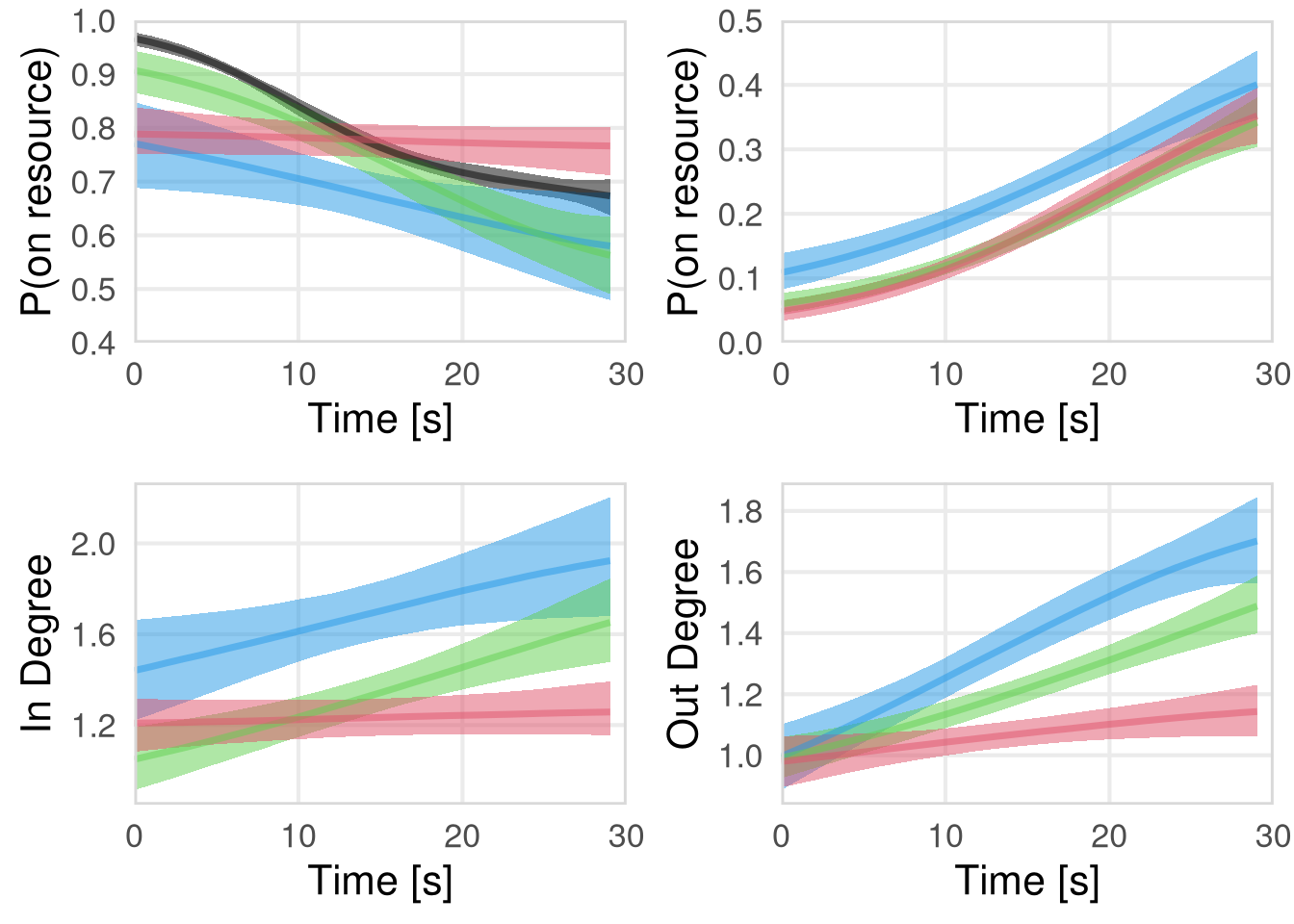
Combine plot (in/out degree full)
resource_discoveries_figure_slow_in_out_full <- ggarrange(
  ggarrange(events_slow_in_degree_fig + scale_y_continuous(limits  = c(0.75, 2.2)), #  + labs(x = "")
            events_slow_outdegree_discoverer_fig + scale_y_continuous(limits  = c(0.35, 1.85)),
            nrow = 2, labels = c("", "")),
  ggarrange(events_slow_in_degree_others_fig + scale_y_continuous(limits  = c(0.75, 2.2)), # + labs(x = "", y = "")
            events_slow_outdegree_fig + scale_y_continuous(limits  = c(0.35, 1.85)),
            nrow = 2, labels = c("", "")),
  ncol = 2,
  widths = c(1, 1)
)

resource_discoveries_figure_slow_in_out_full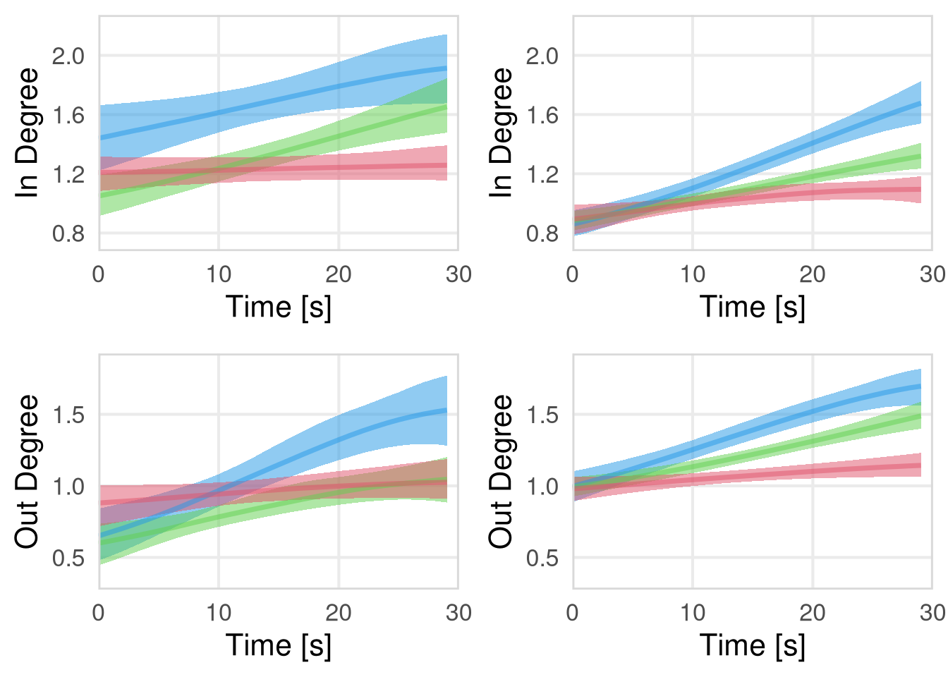
Combine plot VP
resource_discoveries_figure_slow_vp <- ggarrange(
  ggarrange(events_slow_p_stay_vp_fig, events_slow_in_degree_vp_fig, nrow = 2, labels = c("", "")),
  ggarrange(events_slow_p_reach_vp_fig, events_slow_outdegree_vp_fig, nrow = 2, labels = c("", "")),
  ncol = 2,
  widths = c(1, 1)
)

resource_discoveries_figure_slow_vp