Average Median Distance to Resource

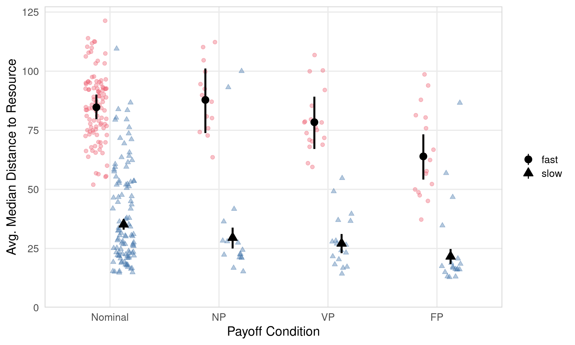
This analysis computes the average median distance to the resource center across the experiment. For each group (or nominal group), at each time step we take the median distance across all members, then average that median across all time steps. We compare this group-level metric between interacting groups (FP, NP, VP) and synthetic “nominal groups” constructed by randomly combining the time-series data of five solitary participants.

Data Preparation

Step 1: Compute per-participant average distance from time series

Step 2: Map participants to groups

Step 3: Compute group-level median distance time series for interacting groups

For interacting groups (FP, NP, VP conditions with valid groups), at each time step we take the median distance across all group members, then average across all time steps.

Step 4: Construct nominal groups from solo participants

We construct synthetic “nominal groups” by randomly combining 5 solitary participants (from the A condition) who played in the same resource speed. For each nominal group, at each time step we take the median across the 5 solo participants’ distances, then average across time.

Step 5: Combine all data

Number of observations per condition:

SignalingType	ResourceSpeed	n
Nominal	fast	500
Nominal	slow	500
FP	fast	17
FP	slow	18
VP	fast	19
VP	slow	17
NP	fast	15
NP	slow	17

Descriptive Statistics

SignalingType	ResourceSpeed	Mean	SD	Median	Min	Max
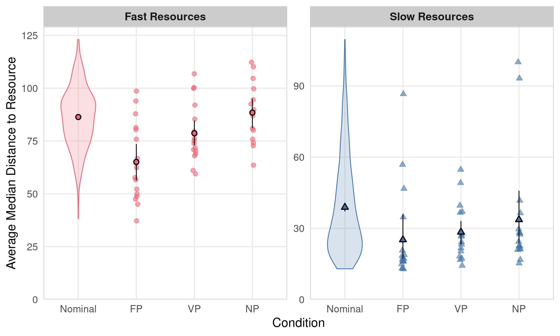
Nominal	fast	86.37	13.98	86.98	38.24	123.01
Nominal	slow	38.87	20.25	32.58	12.95	109.51
FP	fast	65.12	18.33	62.43	37.23	98.64
FP	slow	25.18	19.55	17.01	12.84	86.60
VP	fast	78.69	13.01	76.19	59.49	106.83
VP	slow	28.40	11.49	26.53	14.30	54.74
NP	fast	88.46	14.24	88.54	63.58	112.29
NP	slow	33.65	24.61	24.40	15.28	100.02

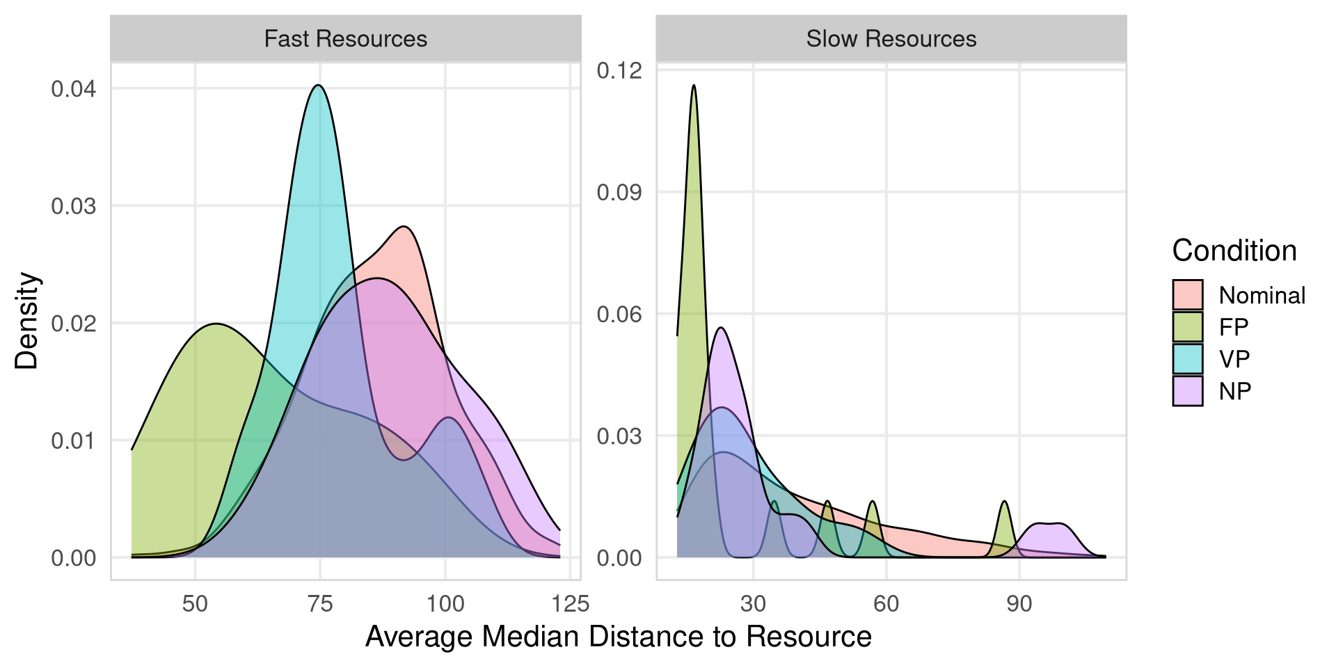
Descriptive Plots

Average Median Distance by Condition

Plot showing the average median distance for nominal groups, FP, VP, and NP, split by resource speed.

Distribution Comparison

Statistical Model

We model the average median distance using a Gamma family with a log link. The dependent variable is a strictly positive, continuous physical distance with a right skew, making the Gamma distribution an appropriate choice. We use SignalingType (Nominal vs FP vs VP vs NP) and ResourceSpeed as predictors with their interaction.

Data for modelling

Real group counts: # A tibble: 2 × 2 ResourceSpeed n 1 fast 51 2 slow 52

m.AvgMedDist.model_data %>%
  ggplot(aes(x = AvgMedDist)) +
  geom_histogram(binwidth = 5, fill = "lightblue", color = "black") +
  facet_grid(rows = vars(ResourceSpeed), cols = vars(SignalingType)) +
  theme_nice()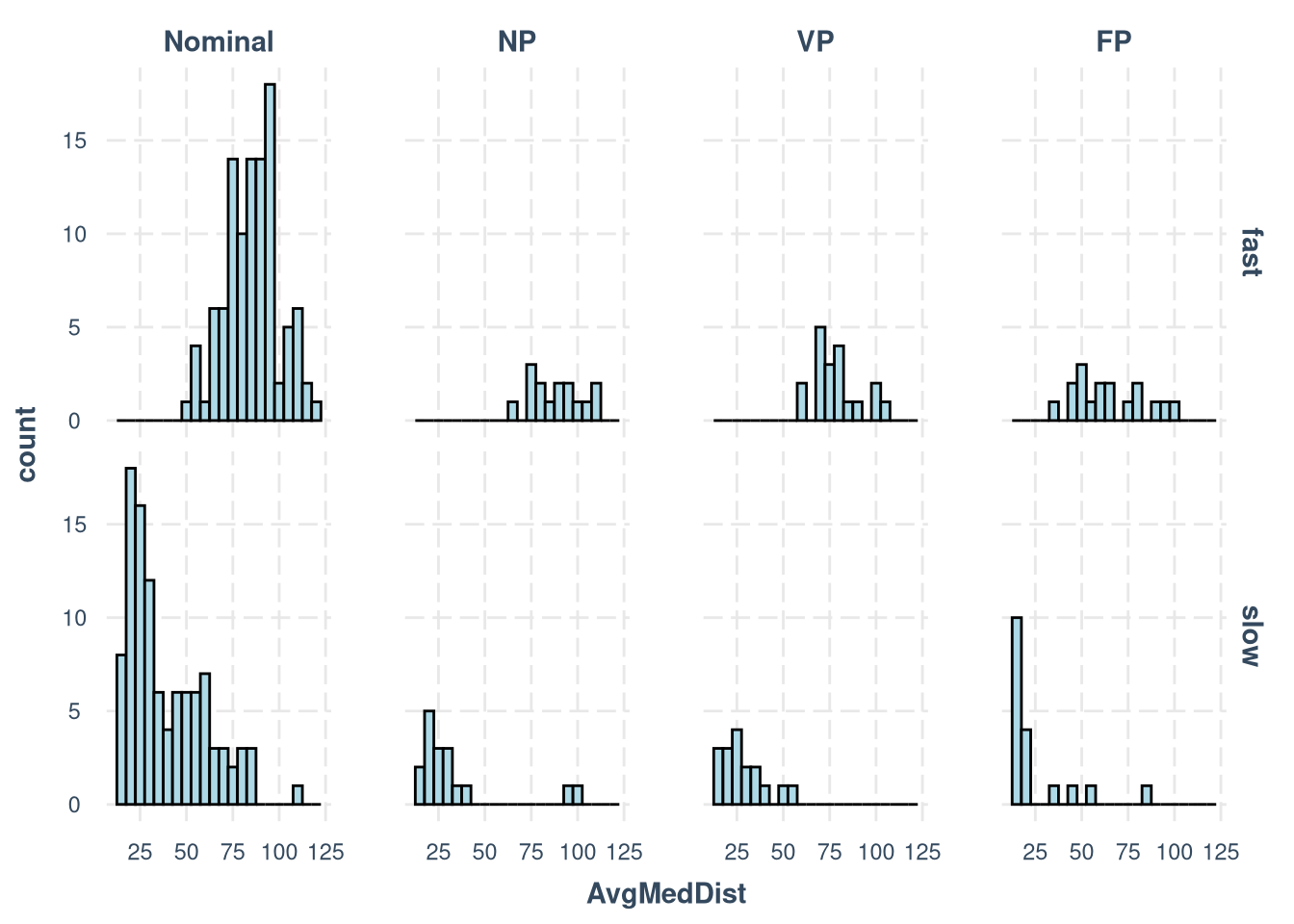

Model specification

m.AvgMedDist.1.formula <- brmsformula(
  AvgMedDist ~ 1 + SignalingType * ResourceSpeed + (1 | Group),
  family = Gamma(link = "log")
)

m.AvgMedDist.1.formula_comparison <- brmsformula(
  AvgMedDist ~ 1 + SignalingType * ResourceSpeed
)

m.AvgMedDist.1.priors <-
  prior(normal(0, 0.5), class = b) +
  prior(normal(4, 1), class = Intercept) + # log(~55) ≈ 4; regularises intercept on log scale
  prior(gamma(4, 0.1), class = shape) +
  prior(exponential(1), class = sd, lb = 0)

Prior predictive checks

m.AvgMedDist.1.fit_prior <- brm(
  formula = m.AvgMedDist.1.formula,
  data = m.AvgMedDist.model_data,
  prior = m.AvgMedDist.1.priors,
  chains = 4,
  cores = 4,
  seed = 42,
  iter = 2000,
  file = paste0(fits_path, "avg_med_dist_1_prior.rds"),
  sample_prior = "only",
  backend = "cmdstanr",
  threads = threading(100),
  control = list(adapt_delta = 0.99),
  save_pars = save_pars(all = TRUE)
)

m.AvgMedDist.1.y <- m.AvgMedDist.model_data$AvgMedDist

summary(m.AvgMedDist.1.fit_prior)

##  Family: gamma 
##   Links: mu = log; shape = identity 
## Formula: AvgMedDist ~ 1 + SignalingType * ResourceSpeed + (1 | Group) 
##    Data: m.AvgMedDist.model_data (Number of observations: 311) 
##   Draws: 4 chains, each with iter = 2000; warmup = 1000; thin = 1;
##          total post-warmup draws = 4000
## 
## Multilevel Hyperparameters:
## ~Group (Number of levels: 311) 
##               Estimate Est.Error l-95% CI u-95% CI Rhat Bulk_ESS Tail_ESS
## sd(Intercept)     1.02      1.01     0.03     3.76 1.00     4115     2157
## 
## Regression Coefficients:
##                                   Estimate Est.Error l-95% CI u-95% CI Rhat Bulk_ESS Tail_ESS
## Intercept                             3.99      1.02     1.98     5.99 1.00     5229     3185
## SignalingTypeNP                       0.00      0.50    -0.96     0.97 1.00     5021     3195
## SignalingTypeVP                       0.00      0.49    -0.96     0.94 1.00     5257     3256
## SignalingTypeFP                      -0.00      0.49    -1.00     0.98 1.00     4869     2933
## ResourceSpeedslow                    -0.01      0.49    -0.97     0.96 1.00     5433     2629
## SignalingTypeNP:ResourceSpeedslow    -0.00      0.51    -1.01     0.98 1.00     4727     3112
## SignalingTypeVP:ResourceSpeedslow     0.00      0.50    -0.97     0.98 1.00     5266     3017
## SignalingTypeFP:ResourceSpeedslow     0.02      0.51    -0.96     1.03 1.00     4915     2912
## 
## Further Distributional Parameters:
##       Estimate Est.Error l-95% CI u-95% CI Rhat Bulk_ESS Tail_ESS
## shape    39.99     20.13    11.02    89.85 1.00     4733     2562
## 
## Draws were sampled using sample(hmc). For each parameter, Bulk_ESS
## and Tail_ESS are effective sample size measures, and Rhat is the potential
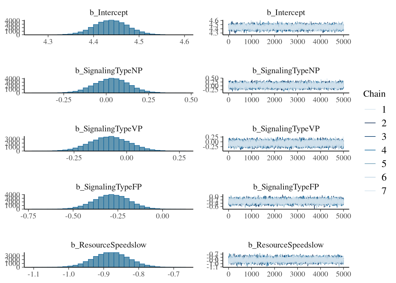
## scale reduction factor on split chains (at convergence, Rhat = 1).

Model fitting

m.AvgMedDist.1.fit <- brm(
  formula = m.AvgMedDist.1.formula,
  data = m.AvgMedDist.model_data,
  prior = m.AvgMedDist.1.priors,
  chains = 7,
  cores = 7,
  seed = 42,
  iter = 10000,
  file = paste0(fits_path, "avg_med_dist_1.rds"),
  backend = "cmdstanr",
  threads = threading(100),
  control = list(adapt_delta = 0.99),
  save_pars = save_pars(all = TRUE)
)

##  Family: gamma 
##   Links: mu = log; shape = identity 
## Formula: AvgMedDist ~ 1 + SignalingType * ResourceSpeed + (1 | Group) 
##    Data: m.AvgMedDist.model_data (Number of observations: 311) 
##   Draws: 7 chains, each with iter = 10000; warmup = 5000; thin = 1;
##          total post-warmup draws = 35000
## 
## Multilevel Hyperparameters:
## ~Group (Number of levels: 311) 
##               Estimate Est.Error l-95% CI u-95% CI Rhat Bulk_ESS Tail_ESS
## sd(Intercept)     0.35      0.02     0.29     0.39 1.00     1341     2721
## 
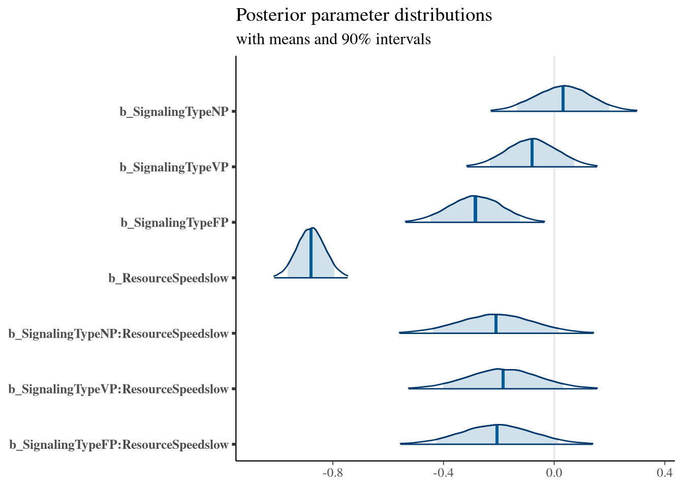
## Regression Coefficients:
##                                   Estimate Est.Error l-95% CI u-95% CI Rhat Bulk_ESS Tail_ESS
## Intercept                             4.44      0.04     4.37     4.51 1.00     7090    13186
## SignalingTypeNP                       0.03      0.10    -0.17     0.23 1.00     7850    14555
## SignalingTypeVP                      -0.08      0.09    -0.26     0.10 1.00     7314    14015
## SignalingTypeFP                      -0.28      0.10    -0.48    -0.10 1.00     7579    12023
## ResourceSpeedslow                    -0.88      0.05    -0.98    -0.78 1.00     7422    13246
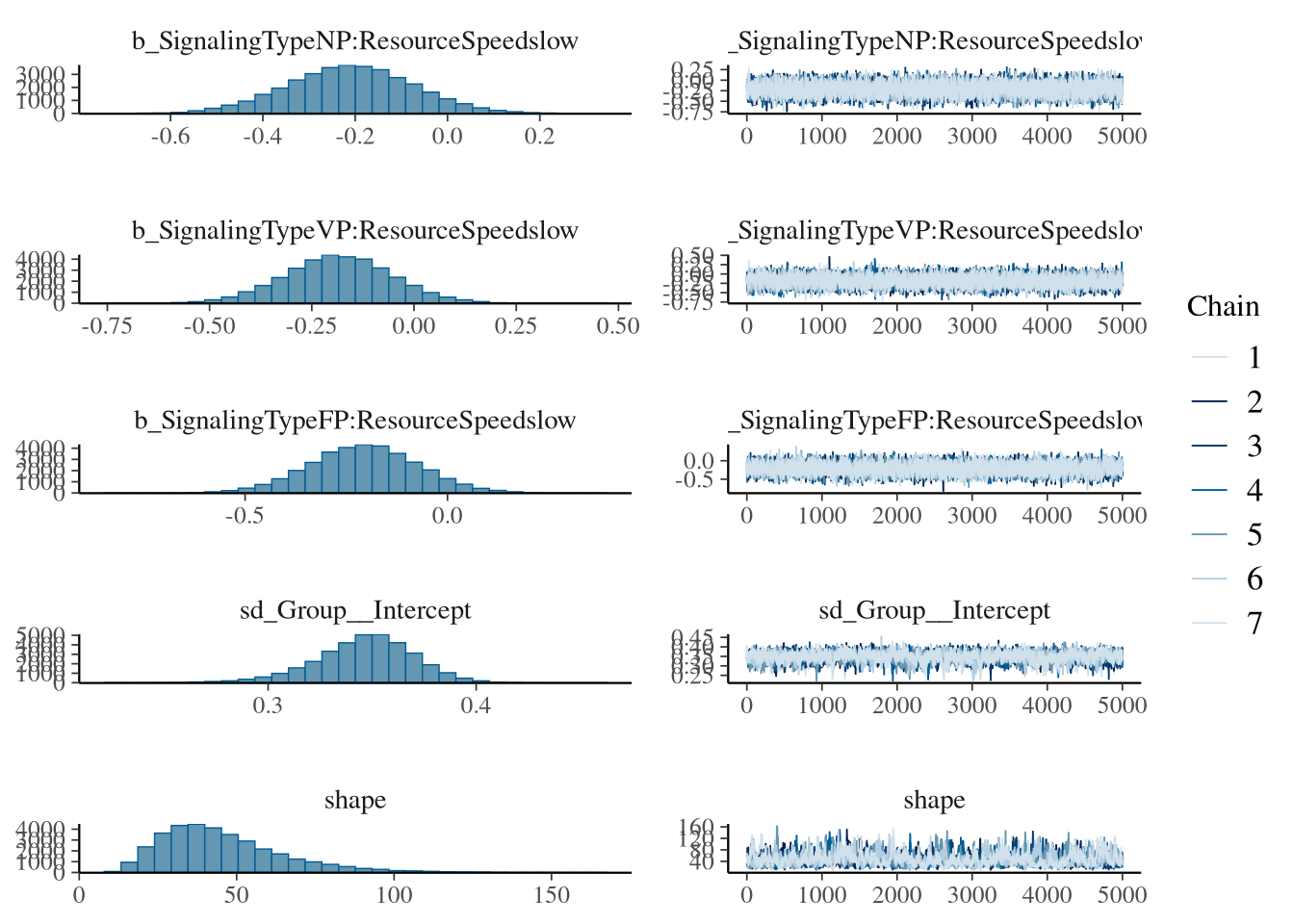
## SignalingTypeNP:ResourceSpeedslow    -0.21      0.14    -0.48     0.06 1.00     8001    13513
## SignalingTypeVP:ResourceSpeedslow    -0.18      0.13    -0.44     0.07 1.00     7636    14063
## SignalingTypeFP:ResourceSpeedslow    -0.21      0.13    -0.47     0.06 1.00     8486    14638
## 
## Further Distributional Parameters:
##       Estimate Est.Error l-95% CI u-95% CI Rhat Bulk_ESS Tail_ESS
## shape    45.47     19.39    18.05    93.12 1.01      792     2017
## 
## Draws were sampled using sample(hmc). For each parameter, Bulk_ESS
## and Tail_ESS are effective sample size measures, and Rhat is the potential
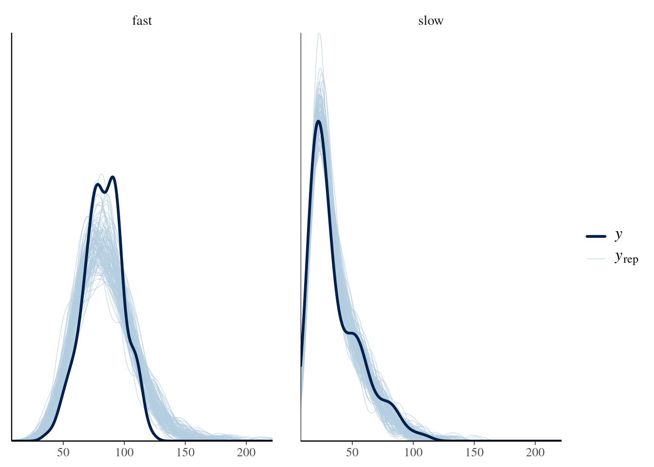
## scale reduction factor on split chains (at convergence, Rhat = 1).

Model diagnostics

m.AvgMedDist.1.yrep <- posterior_predict(m.AvgMedDist.1.fit, draws = 1000)

plot(m.AvgMedDist.1.fit, ask = FALSE)

ppc_dens_overlay(m.AvgMedDist.1.y, m.AvgMedDist.1.yrep[1:100, ])

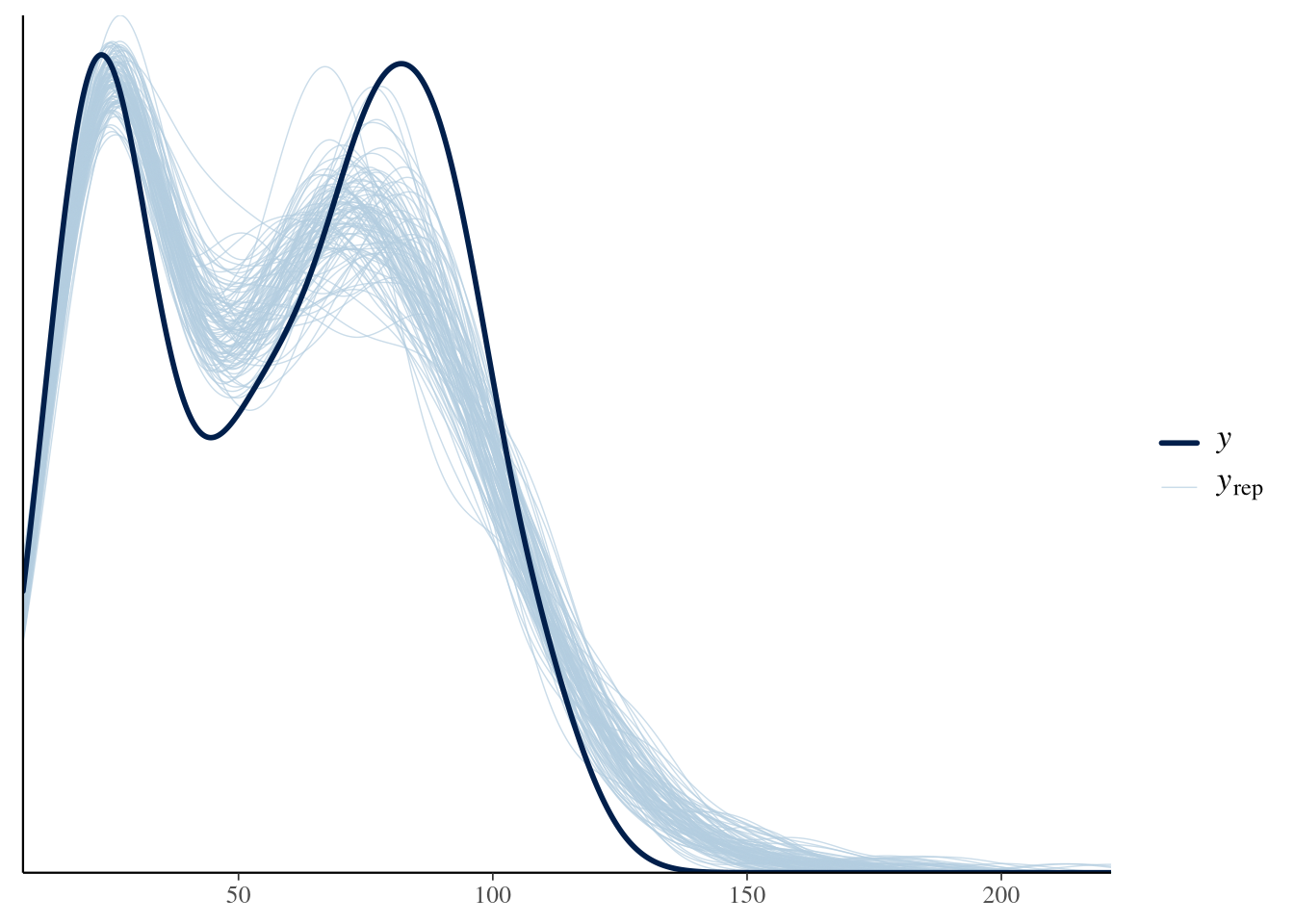
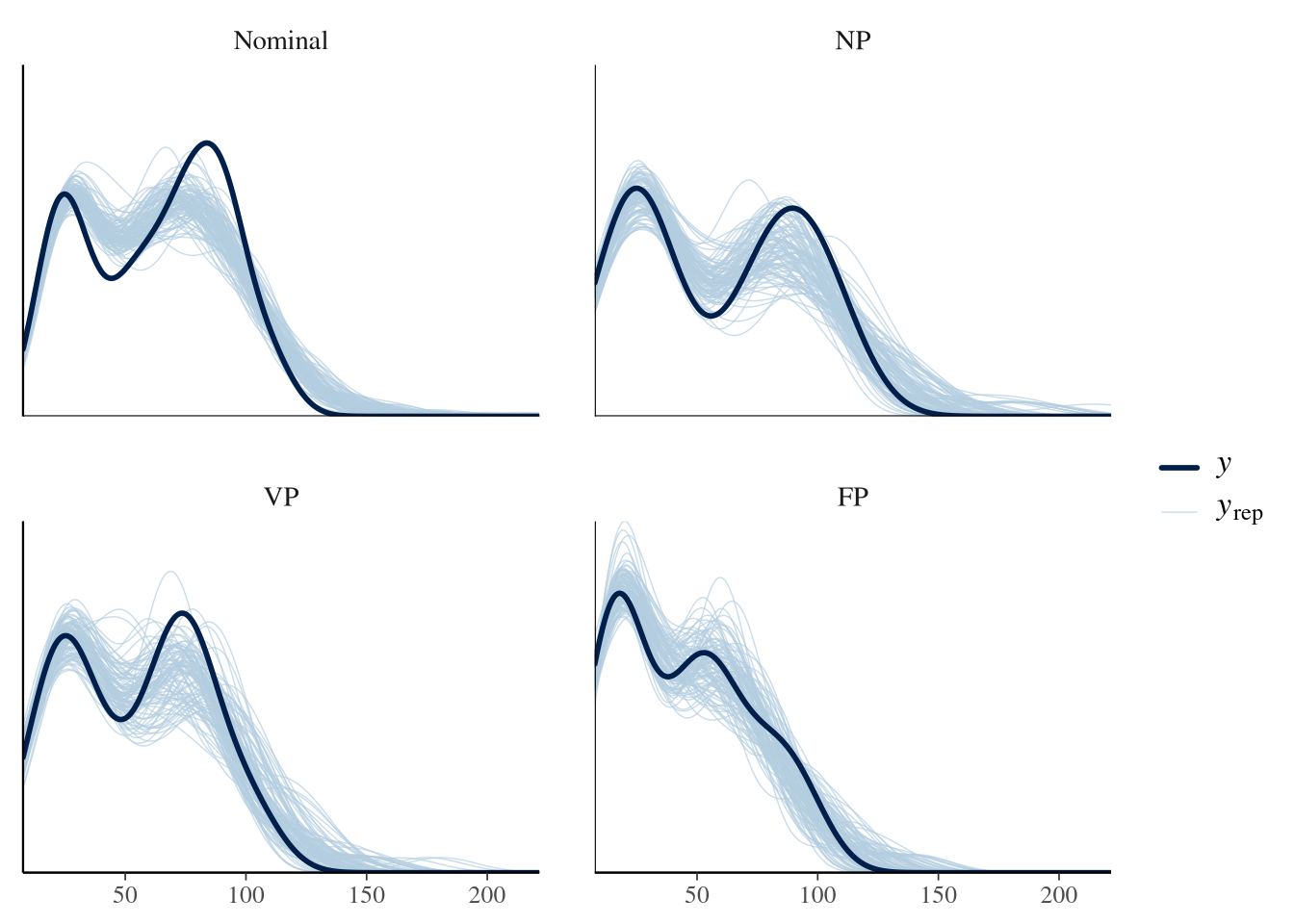
ppc_dens_overlay_grouped(m.AvgMedDist.1.y, m.AvgMedDist.1.yrep[1:100, ],
  group = m.AvgMedDist.model_data$ResourceSpeed
)

ppc_dens_overlay_grouped(m.AvgMedDist.1.y, m.AvgMedDist.1.yrep[1:100, ],
  group = m.AvgMedDist.model_data$SignalingType
)

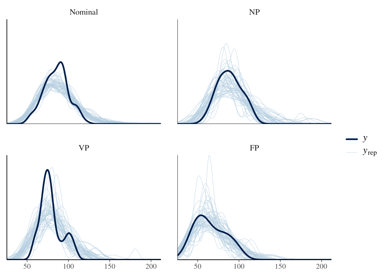
group <- m.AvgMedDist.model_data$SignalingType
mask <- m.AvgMedDist.model_data$ResourceSpeed == "fast"

ppc_dens_overlay_grouped(m.AvgMedDist.1.y[mask],
  m.AvgMedDist.1.yrep[1:50, mask],
  group = group[mask]
)

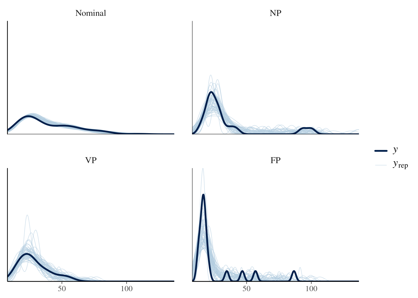
group <- m.AvgMedDist.model_data$SignalingType
mask <- m.AvgMedDist.model_data$ResourceSpeed == "slow"

ppc_dens_overlay_grouped(m.AvgMedDist.1.y[mask],
  m.AvgMedDist.1.yrep[1:50, mask],
  group = group[mask]
)

Model predictions

Condition comparisons

m.AvgMedDist.1.emmeans_contrast_draws.1 <- m.AvgMedDist.1.fit %>%
  emmeans(~ SignalingType * ResourceSpeed,
    epred = TRUE,
    type = "response",
    re_formula = m.AvgMedDist.1.formula_comparison
  ) %>%
  contrast(method = "pairwise", simple = "each", combine = TRUE) %>%
  gather_emmeans_draws()

m.AvgMedDist.1.comparison.1 <- m.AvgMedDist.1.emmeans_contrast_draws.1 %>%
  ggdist::mean_hdci(.width = 0.9) %>%
  mutate(.value = round(.value, 2), .lower = round(.lower, 2), .upper = round(.upper, 2))

m.AvgMedDist.1.comparison.1 %>%
  knitr::kable("html", digits = 2) %>%
  kable_classic(full_width = TRUE, position = "center")

ResourceSpeed	SignalingType	contrast	.value	.lower	.upper	.width	.point	.interval
.	FP	fast - slow	42.35	32.35	52.22	0.9	mean	hdci
.	Nominal	fast - slow	49.53	44.05	55.03	0.9	mean	hdci
.	NP	fast - slow	58.30	43.69	72.19	0.9	mean	hdci
.	VP	fast - slow	51.32	39.28	62.57	0.9	mean	hdci
fast	.	Nominal - FP	20.77	9.91	31.46	0.9	mean	hdci
fast	.	Nominal - NP	-3.12	-16.94	12.08	0.9	mean	hdci
fast	.	Nominal - VP	6.31	-5.91	18.21	0.9	mean	hdci
fast	.	NP - FP	23.89	6.55	40.48	0.9	mean	hdci
fast	.	NP - VP	9.43	-8.14	27.00	0.9	mean	hdci
fast	.	VP - FP	14.46	0.03	29.33	0.9	mean	hdci
slow	.	Nominal - FP	13.58	9.69	17.35	0.9	mean	hdci
slow	.	Nominal - NP	5.65	0.96	10.70	0.9	mean	hdci
slow	.	Nominal - VP	8.09	3.66	12.74	0.9	mean	hdci
slow	.	NP - FP	7.93	2.40	13.34	0.9	mean	hdci
slow	.	NP - VP	2.44	-3.73	8.32	0.9	mean	hdci
slow	.	VP - FP	5.49	0.34	10.66	0.9	mean	hdci

m.AvgMedDist.1.emmeans_contrast_draws.1 %>%
  filter(ResourceSpeed != ".") %>%
  rename(prediction = .value) %>%
  ggplot(
    aes(
      y = contrast,
      x = prediction,
      color = ResourceSpeed, shape = ResourceSpeed, fill = ResourceSpeed
    )
  ) +
  facet_grid(rows = vars(ResourceSpeed)) +
  stat_pointinterval(.width = 0.9) +
  scale_color_manual(values = get_colors("Qual2", num.colors = 2, reverse = TRUE, gradient = FALSE)) +
  scale_fill_manual(values = get_colors("Qual2", num.colors = 2, reverse = TRUE, gradient = FALSE)) +
  scale_shape_manual(values = c(21, 24)) +
  geom_vline(aes(xintercept = 0), linetype = "longdash") +
  labs(x = "Difference in Average Median Distance") +
  theme_nice()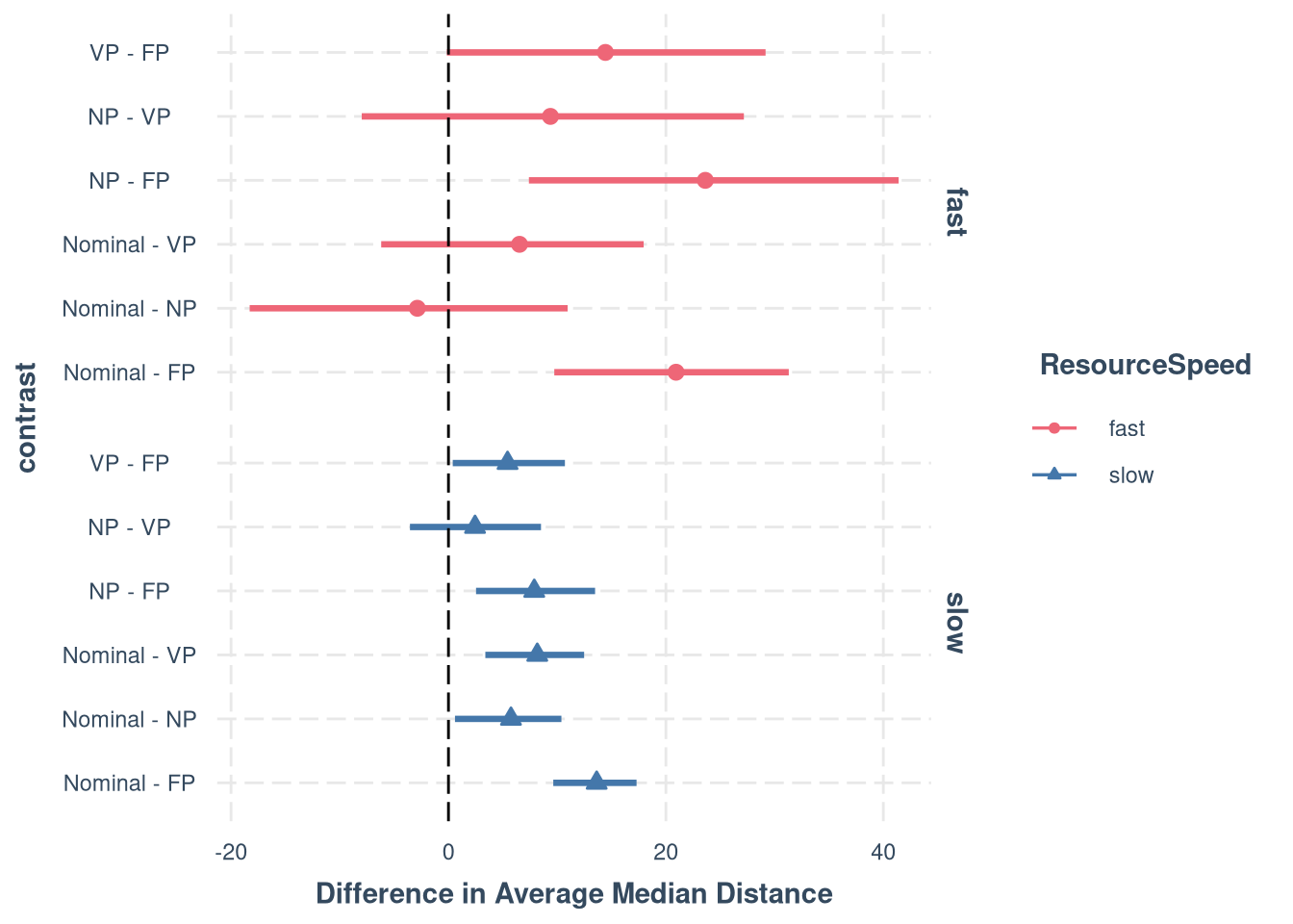

m.AvgMedDist.1.emmeans_contrast_draws.2 <- m.AvgMedDist.1.fit %>%
  emmeans(~ResourceSpeed,
    epred = TRUE,
    type = "response",
    re_formula = m.AvgMedDist.1.formula_comparison
  ) %>%
  contrast(method = "pairwise", simple = "each", combine = TRUE) %>%
  gather_emmeans_draws()

m.AvgMedDist.1.comparison.2 <- m.AvgMedDist.1.emmeans_contrast_draws.2 %>%
  ggdist::mean_hdci(.width = 0.9) %>%
  mutate(.value = round(.value, 2), .lower = round(.lower, 2), .upper = round(.upper, 2))

m.AvgMedDist.1.comparison.2 %>%
  knitr::kable("html", digits = 2) %>%
  kable_classic(full_width = TRUE, position = "center")

contrast	.value	.lower	.upper	.width	.point	.interval
fast - slow	50.38	44.93	55.87	0.9	mean	hdci

Combined comparison table

m.AvgMedDist.1.comparison.combined_table <- bind_rows(
  m.AvgMedDist.1.comparison.2,
  m.AvgMedDist.1.comparison.1
) %>%
  select(ResourceSpeed, SignalingType, contrast, .value, .lower, .upper) %>%
  mutate(
    ResourceSpeed = ifelse(is.na(ResourceSpeed), ".", as.character(ResourceSpeed)),
    SignalingType = ifelse(is.na(SignalingType), ".", as.character(SignalingType)),
    sig = (.lower * .upper) > 0,
    Estimate = sprintf("%.2f", .value),
    Estimate = ifelse(sig, paste0("\\textbf{", Estimate, "}"), Estimate),
    hpdi = sprintf("[%.2f, %.2f]", .lower, .upper),
    hpdi = ifelse(sig, paste0("\\textbf{", hpdi, "}"), hpdi)
  ) %>%
  select(ResourceSpeed, SignalingType, contrast, Estimate, hpdi)

colnames(m.AvgMedDist.1.comparison.combined_table) <- c(
  "Resource Speed", "Payoff Condition", "Contrast", "Mean", "90\\% HPDI"
)


kbl <- kable(
  m.AvgMedDist.1.comparison.combined_table,
  format = "latex",
  booktabs = TRUE,
  align = c("l", "l", "l", "r", "r"),
  caption = "Posterior Estimates Average Median Distance",
  escape = FALSE
) %>%
  kable_styling(latex_options = "hold_position") %>%
  row_spec(0, bold = TRUE)

unique_speeds <- unique(m.AvgMedDist.1.comparison.combined_table$`Resource Speed`)
start <- 1
for (speed in unique_speeds) {
  n_rows <- sum(m.AvgMedDist.1.comparison.combined_table$`Resource Speed` == speed)
  if (speed != ".") {
    kbl <- group_rows(kbl, speed, start, start + n_rows - 1)
  }
  start <- start + n_rows
}

writeLines(kbl, paste0(comparisons, "avg_med_dist_1_comparison_combined.tex"))

Collective Resource Tracking Statistical Analysis