Voluntary Payoff Sharing
m.PayoffSharing.data <- time_series_data %>%
  filter(SignalingType == 'VP') %>%
  filter(State != 'mixed') %>%
  mutate(
    c_OwnDistFromResource = OwnDistFromResource / 40,
    c_Time = Time / max(Time)
  ) %>%
  mutate(State = case_when(State == 'tracking' ~ 'Tracking',
                           State == 'searching' ~ 'Searching')) %>%
  mutate(State = relevel(as.factor(State), ref = "Tracking")) %>%
  select(Participant, ResourceSpeed, State, IsSignaling, Time, c_Time, OwnDistFromResource,
         c_OwnDistFromResource)


head(m.PayoffSharing.data)
m.PayoffSharing.data %>%
group_by(Participant) %>%
summarise(payoff_sharing_probability = mean(IsSignaling), ResourceSpeed = unique(ResourceSpeed)) %>%
ggplot(aes(x=payoff_sharing_probability)) +
geom_histogram(alpha=0.5, binwidth = 0.05) +
# geom_density() +
facet_grid(cols=vars(ResourceSpeed)) +
theme_nice() +
labs(x = "Proportion of Time")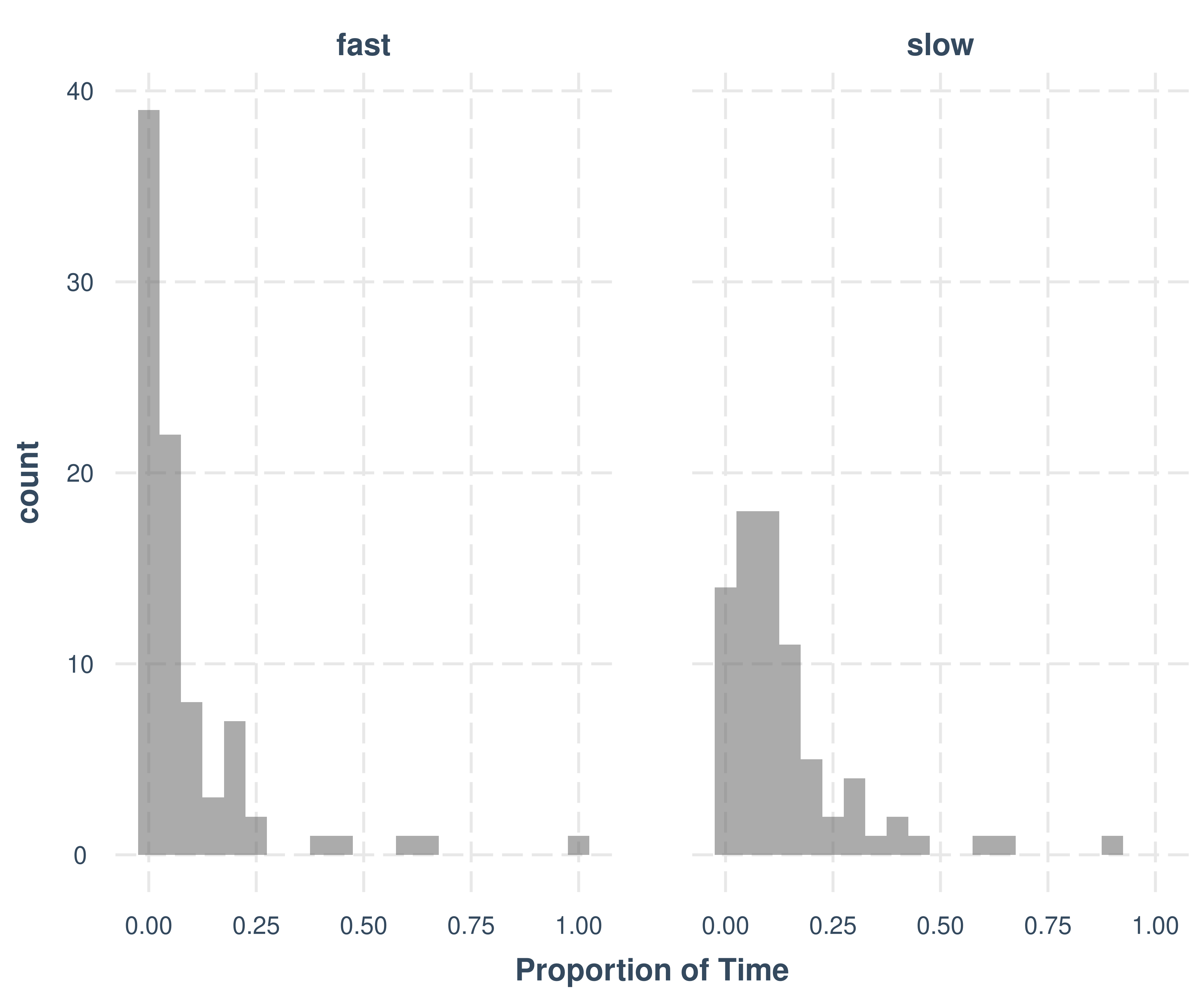
# Step 1: participant means
m.PayoffSharing.data %>%
  group_by(Participant, ResourceSpeed) %>%
  summarise(payoff_sharing_probability = mean(IsSignaling, na.rm = TRUE),
            .groups = "drop") %>%  # Step 2: grand mean and SD across participants
  group_by(ResourceSpeed) %>%
  summarise(
    mean_probability = mean(payoff_sharing_probability),
    sd_probability = sd(payoff_sharing_probability),
    n = n()
  )
m.PayoffSharing.data %>%
filter(State == "Tracking", OwnDistFromResource < 10) %>%
group_by(Participant) %>%
summarise(payoff_sharing_probability = mean(IsSignaling), ResourceSpeed = unique(ResourceSpeed),
n = n()) %>%
filter(n > 10) %>%
ggplot(aes(x=payoff_sharing_probability)) +
geom_histogram(alpha=0.5, binwidth = 0.01) +
geom_density() +
facet_grid(cols=vars(ResourceSpeed)) +
theme_nice() +
labs(title = "Distribution of Payoff Sharing Probabilities",
subtitle = "groupped by participant",
x = "Payoff Sharing Probability (Proportion of Time)")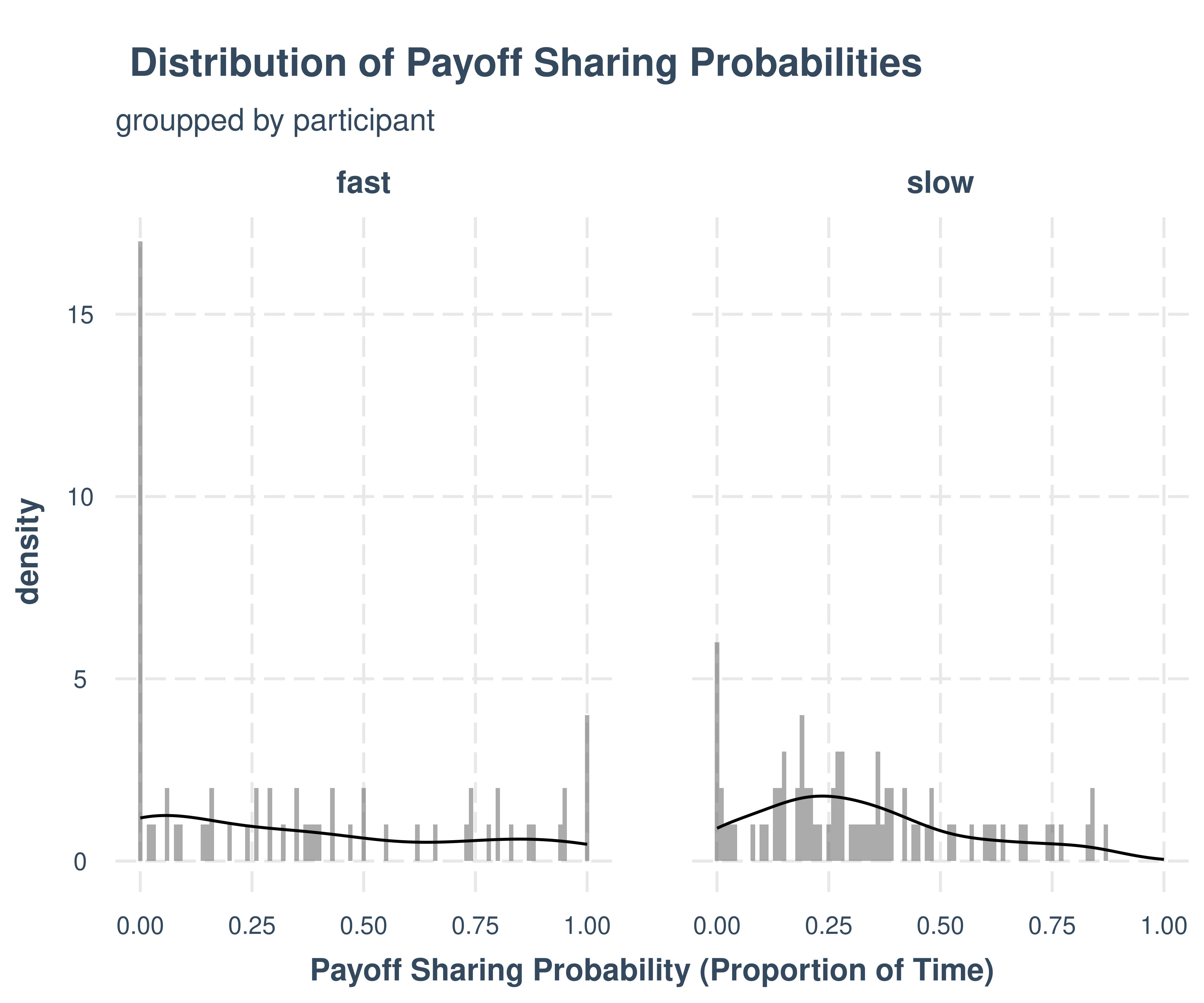
Sharing actions count
switch_counts <- m.PayoffSharing.data %>%
  arrange(Participant, Time) %>%
  group_by(Participant) %>%  # , State
  summarise(
    n_switch_0_to_1 = sum(
      lag(IsSignaling) == 0 &
      IsSignaling == 1 &
      Time == lag(Time) + 1,
      na.rm = TRUE
    ),
    .groups = "drop"
  )

hist(switch_counts$n_switch_0_to_1)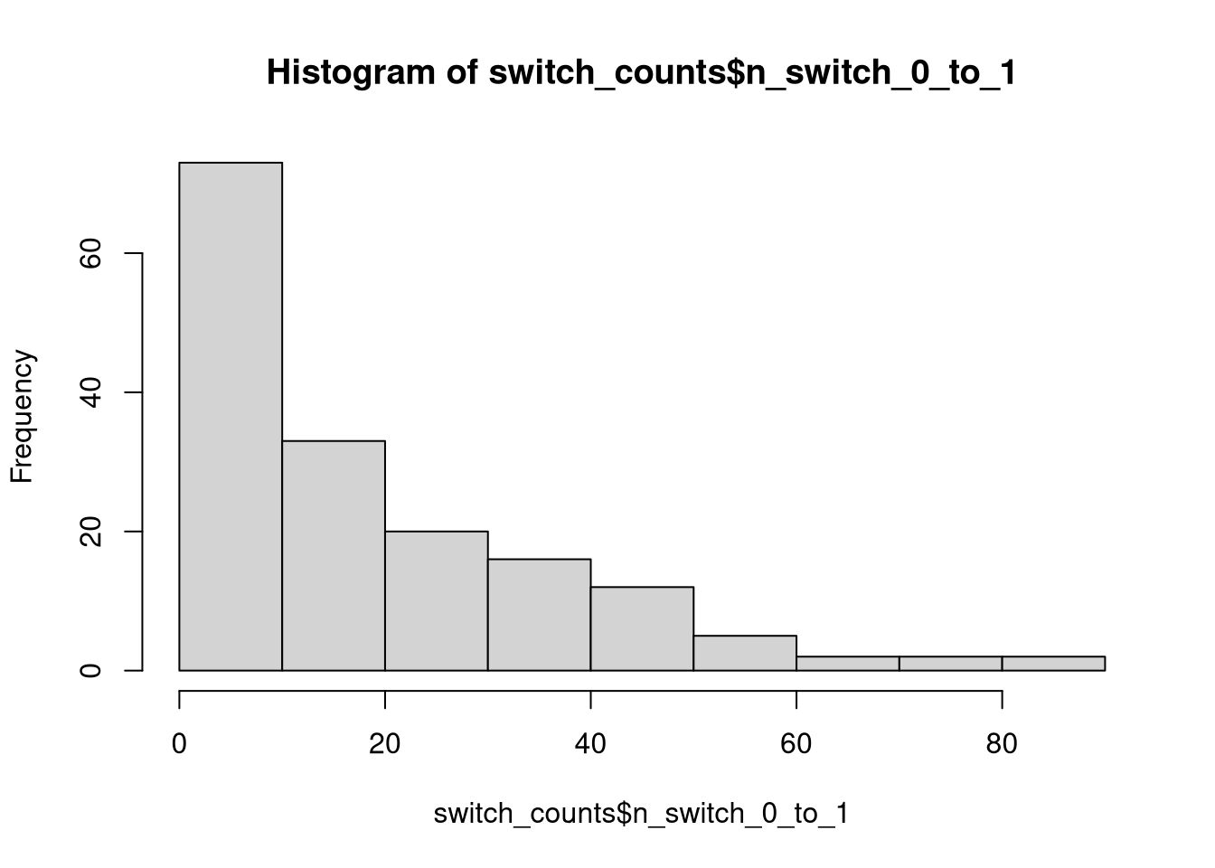
m.PayoffSharing.SwitchCounts.data <- subj_data %>%
  filter(SignalingType == 'VP') %>%
  select(Participant, Group, ResourceSpeed, SignalingType, PCR, Score, TrackingTime) %>%
  left_join(switch_counts, by = "Participant") %>%
  mutate(PCR_0_1 = PCR / 40,
         Score_0_1 = Score / empirical_max_score,
         TrackingTime_0_1 = TrackingTime / 15.01,
         c_n_switch_0_to_1 = n_switch_0_to_1 / max(n_switch_0_to_1))
m.PayoffSharing.SwitchCounts.data %>%
dplyr::summarize(
n = n(),
n_never_signaled = sum(n_switch_0_to_1 == 0),
precentage_never_signaled = round((n_never_signaled / n) * 100, 2),
signaled_once = sum(n_switch_0_to_1 == 1)
)m.PayoffSharing.SwitchCounts.data %>%
group_by(ResourceSpeed) %>%
dplyr::summarize(
n = n(),
n_never_signaling = sum(n_switch_0_to_1 == 0)
)Count Model
m.PayoffSharing.SwitchCounts.formula <- brmsformula(
  n_switch_0_to_1 ~ ResourceSpeed + (1 | Participant),
  family = poisson()
  )

m.PayoffSharing.SwitchCounts.priors <-
    prior(normal(0, 0.5), class = b) +
    prior(normal(0, 0.1), class = 'sd') +
    prior(normal(0, 1), class = Intercept)
Model fitting
m.PayoffSharing.SwitchCounts.fit <- brm(
  formula = m.PayoffSharing.SwitchCounts.formula,
  data    = m.PayoffSharing.SwitchCounts.data,
  prior   = m.PayoffSharing.SwitchCounts.priors,
  chains  = 4,
  cores   = 4,
  seed    = 42,
  iter    = 2000,
  file = paste0(fits_path, 'payoff_sharing_count_1.rds'),
  backend = "cmdstanr",
  threads = threading(100),
  control = list(adapt_delta = 0.95),
  save_pars = save_pars(all = TRUE)
  )
Model diagnostics
##  Family: poisson
##   Links: mu = log
## Formula: n_switch_0_to_1 ~ ResourceSpeed + (1 | Participant)
##    Data: m.PayoffSharing.SwitchCounts.data (Number of observations: 165)
##   Draws: 4 chains, each with iter = 2000; warmup = 1000; thin = 1;
##          total post-warmup draws = 4000
##
## Multilevel Hyperparameters:
## ~Participant (Number of levels: 165)
##               Estimate Est.Error l-95% CI u-95% CI Rhat Bulk_ESS Tail_ESS
## sd(Intercept)     0.76      0.04     0.68     0.85 1.00     1456     1899
##
## Regression Coefficients:
##                   Estimate Est.Error l-95% CI u-95% CI Rhat Bulk_ESS Tail_ESS
## Intercept             1.88      0.09     1.70     2.05 1.00     1269     2332
## ResourceSpeedslow     1.15      0.13     0.91     1.40 1.00      582     1525
##
## Draws were sampled using sample(hmc). For each parameter, Bulk_ESS
## and Tail_ESS are effective sample size measures, and Rhat is the potential
## scale reduction factor on split chains (at convergence, Rhat = 1).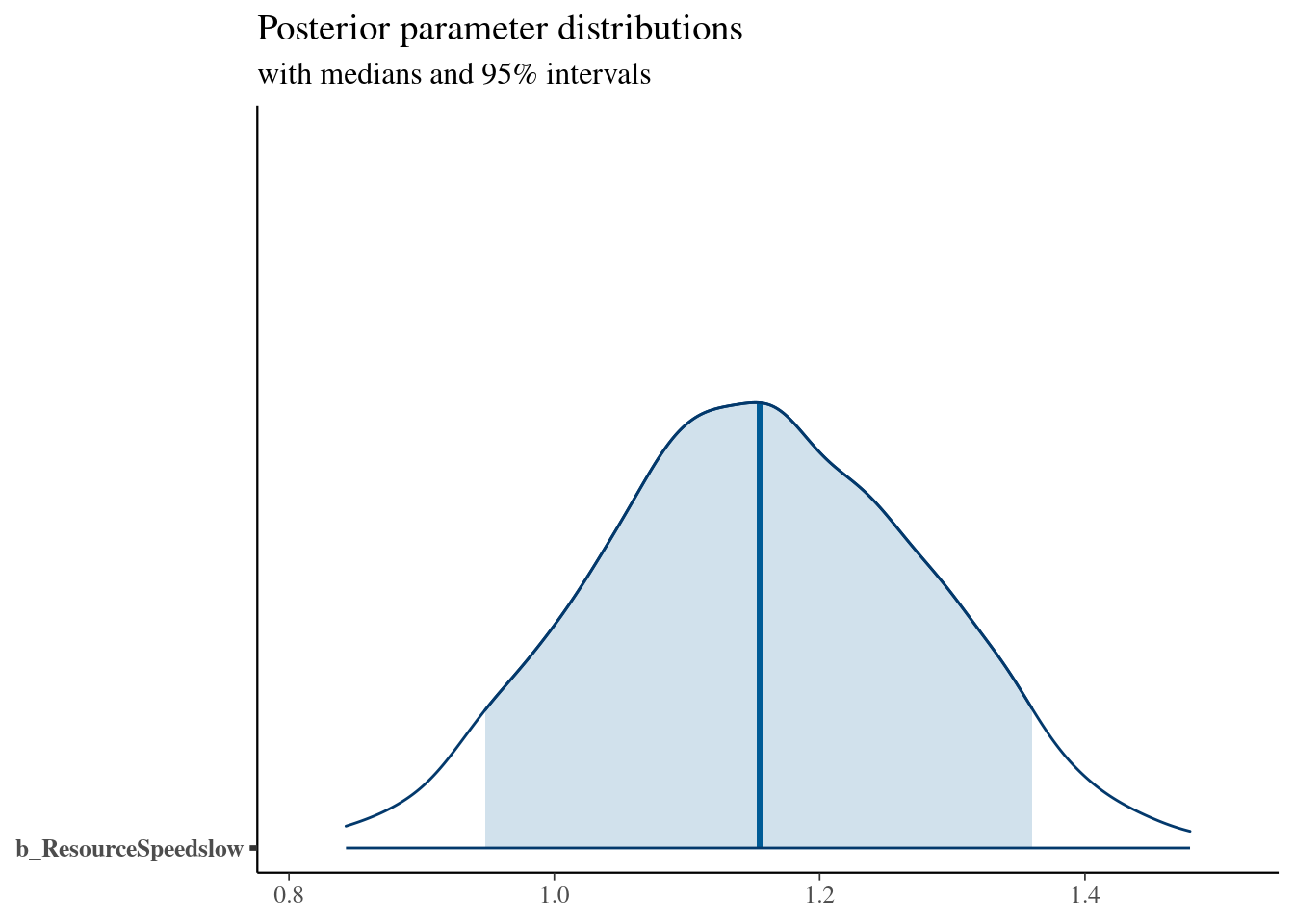
Condition draws
m.PayoffSharing.SwitchCounts.fit %>%
  emmeans(~ ResourceSpeed, epred = TRUE, type = "response", re_formula = NA) %>%
  gather_emmeans_draws() %>%
  ggdist::mean_hdci(.width = 0.9) %>%
knitr::kable("html", digits = 2) %>% kable_classic(full_width = T, position = "center", )| ResourceSpeed | .value | .lower | .upper | .width | .point | .interval |
|---|---|---|---|---|---|---|
| fast | 6.58 | 5.60 | 7.59 | 0.9 | mean | hdci |
| slow | 20.88 | 17.79 | 23.96 | 0.9 | mean | hdci |
Count vs Score model
m.PayoffSharing.SwitchCounts.data %>%
  ggplot(aes(x=n_switch_0_to_1, y=Score, color=ResourceSpeed)) +
  facet_wrap(vars(ResourceSpeed), scales="free") +
  geom_point() +
  geom_smooth(method="lm")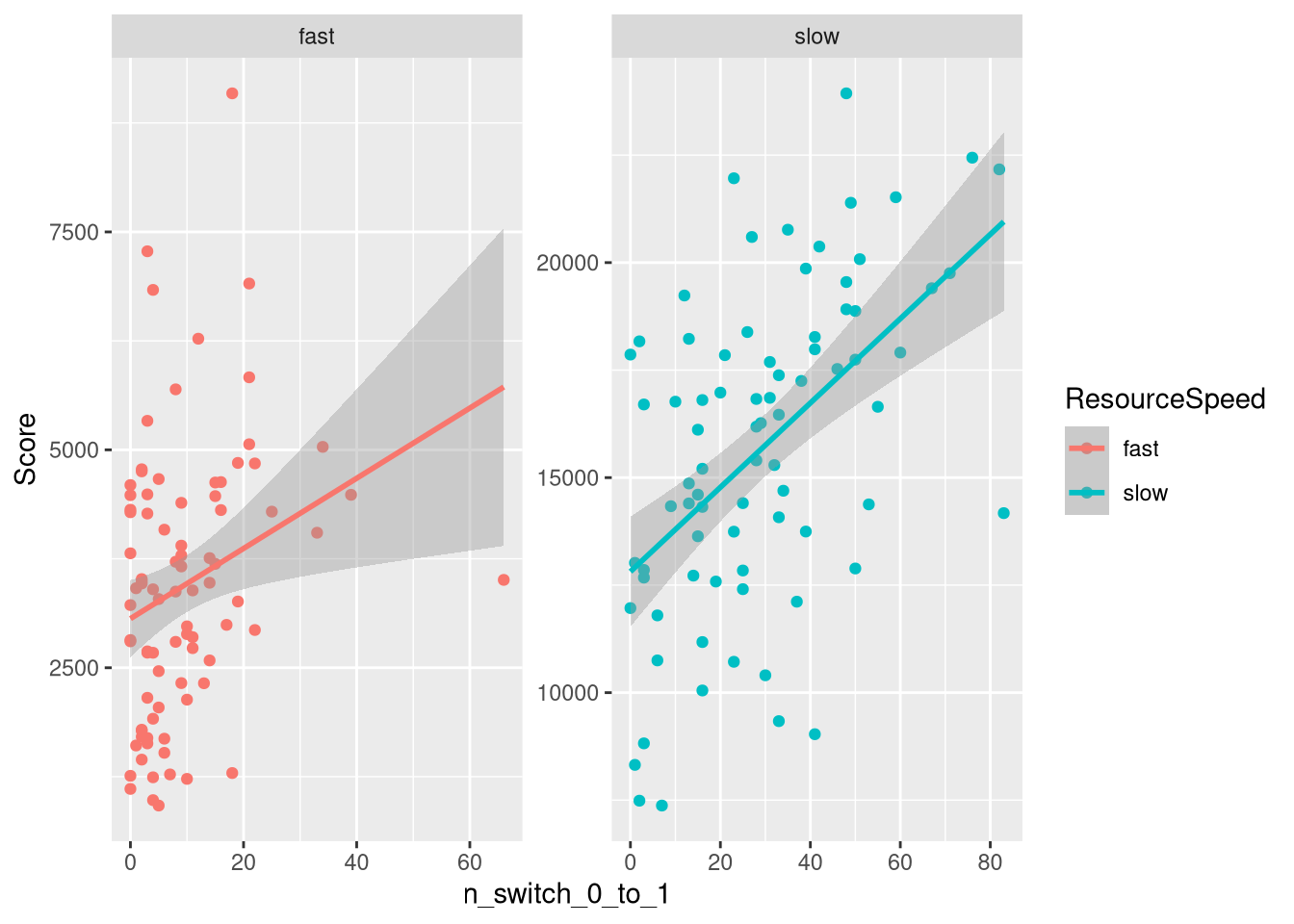
m.PayoffSharing.SwitchCounts.data %>%
  group_by(Group) %>%
  summarise(
    Score_0_1 = mean(Score),
    TrackingTime_0_1 = mean(TrackingTime_0_1),
    PCR_0_1 = mean(PCR_0_1),
    sum_n_switch_0_to_1 = sum(n_switch_0_to_1),
    ResourceSpeed = unique(ResourceSpeed)
  ) %>%
  mutate(sum_n_switch_0_to_1 = sum_n_switch_0_to_1 / max(sum_n_switch_0_to_1)) %>%
  ggplot(aes(x=sum_n_switch_0_to_1, y=Score_0_1, color=ResourceSpeed)) +
  facet_wrap(vars(ResourceSpeed), scales="free") +
  geom_point() +
  geom_smooth(method="lm")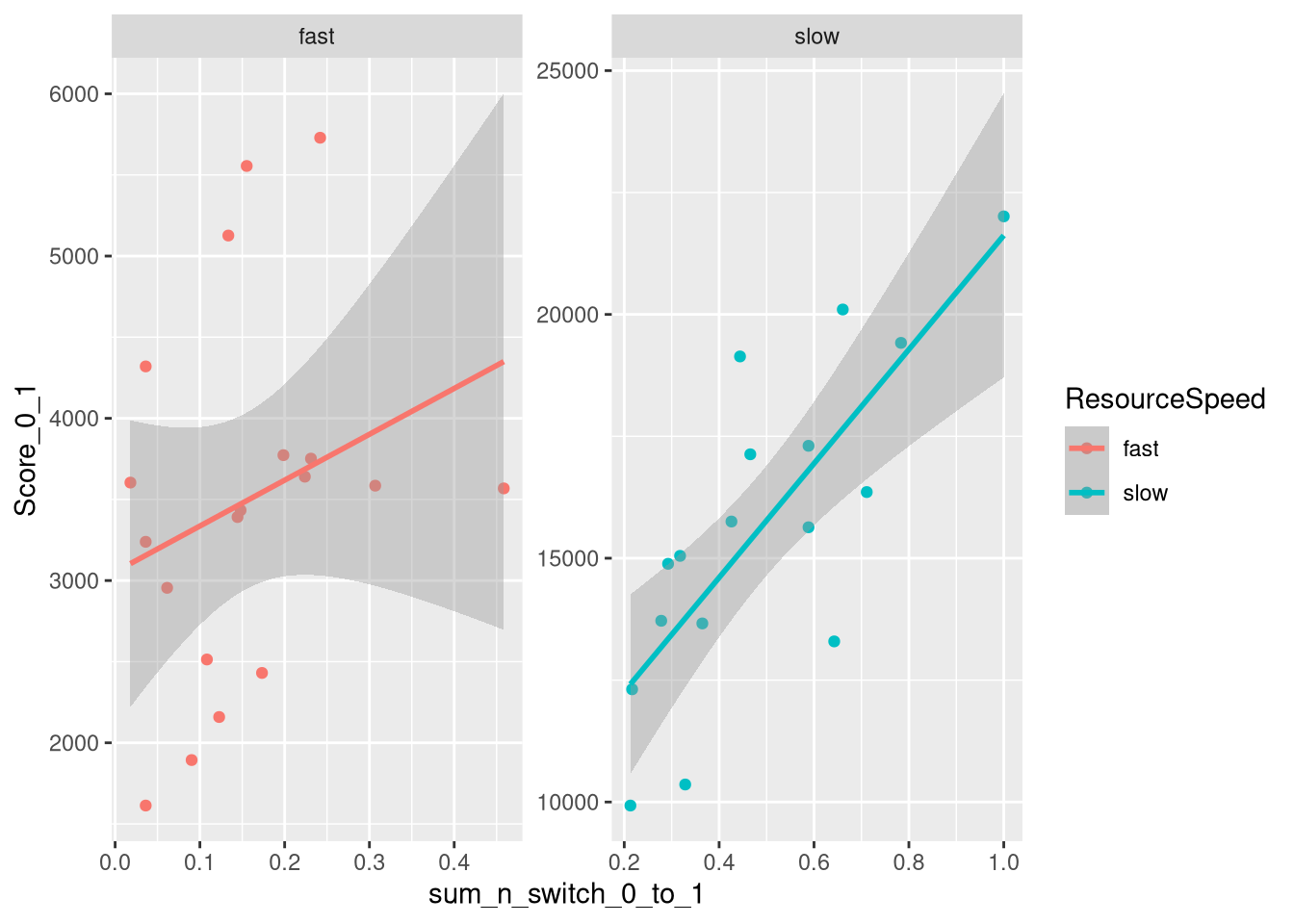
Model fitting (Participant)
m.PayoffSharing.SwitchCounts.Score.formula <- brmsformula(
  Score_0_1 ~ ResourceSpeed * c_n_switch_0_to_1,
  phi ~ ResourceSpeed,
  family = Beta()
)

m.PayoffSharing.SwitchCounts.Score.priors <-
    prior(normal(0, 0.5), class = b) +
    prior(normal(0, 1), class = Intercept) +
    prior(gamma(4, 0.1), class = Intercept, dpar = phi, lb = 0)
m.PayoffSharing.SwitchCounts.Score.fit <- brm(
formula = m.PayoffSharing.SwitchCounts.Score.formula,
data = m.PayoffSharing.SwitchCounts.data,
prior = m.PayoffSharing.SwitchCounts.Score.priors,
chains = 4,
cores = 4,
seed = 42,
iter = 2000,
file = paste0(fits_path, 'pyoff_sharing_count_score.rds'),
backend = "cmdstanr",
threads = threading(100),
save_pars = save_pars(all = TRUE)
)Model diagnostics
##  Family: beta
##   Links: mu = logit; phi = log
## Formula: Score_0_1 ~ ResourceSpeed * c_n_switch_0_to_1
##          phi ~ ResourceSpeed
##    Data: m.PayoffSharing.SwitchCounts.data (Number of observations: 165)
##   Draws: 4 chains, each with iter = 2000; warmup = 1000; thin = 1;
##          total post-warmup draws = 4000
##
## Regression Coefficients:
##                                     Estimate Est.Error l-95% CI u-95% CI Rhat Bulk_ESS Tail_ESS
## Intercept                              -1.93      0.06    -2.06    -1.81 1.00     3327     3362
## phi_Intercept                           3.45      0.15     3.14     3.75 1.00     3814     2712
## ResourceSpeedslow                       1.88      0.11     1.66     2.10 1.00     3294     2868
## c_n_switch_0_to_1                       0.79      0.27     0.26     1.30 1.00     2838     2712
## ResourceSpeedslow:c_n_switch_0_to_1     0.63      0.31     0.04     1.23 1.00     2635     2483
## phi_ResourceSpeedslow                  -0.84      0.22    -1.27    -0.41 1.00     3944     3009
##
## Draws were sampled using sample(hmc). For each parameter, Bulk_ESS
## and Tail_ESS are effective sample size measures, and Rhat is the potential
## scale reduction factor on split chains (at convergence, Rhat = 1).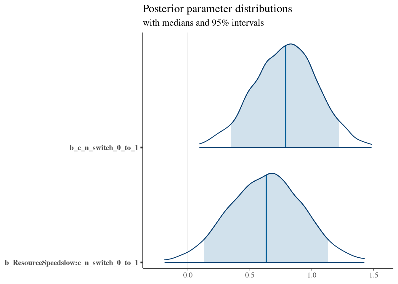
Figure
fig_payoff_sharing_switch_count_score <- m.PayoffSharing.SwitchCounts.data %>%
  select(Participant, ResourceSpeed, c_n_switch_0_to_1) %>%
  group_by() %>%
  data_grid(ResourceSpeed, c_n_switch_0_to_1=seq(0, 1, 0.1)) %>%
  tidybayes::add_epred_draws(m.PayoffSharing.SwitchCounts.Score.fit,
                             allow_new_levels = TRUE,
                             re_formula = NA) %>%
  ggplot(aes(x = c_n_switch_0_to_1 * max(m.PayoffSharing.SwitchCounts.data$n_switch_0_to_1),
             y = .epred * empirical_max_score,
             color = ResourceSpeed,
             fill = ResourceSpeed)) +
  stat_lineribbon(aes(group = paste(group, ...width..)), .width = c(.9), alpha = 0.5) +
  scale_color_manual(breaks = c('fast', 'slow'),
                     aesthetics = c("colour", "fill"),
                    values = get_colors("Qual2", num.colors = 2, reverse = TRUE, gradient = FALSE),
                    guide = guide_legend(
                    title = "Resource",
                     )
                    ) +
  geom_point(
    data = m.PayoffSharing.SwitchCounts.data,
    aes(x = n_switch_0_to_1, y = Score),  # , color = ResourceSpeed
    color = 'black',
    inherit.aes = FALSE,
    alpha = 0.45,
    size = 1.6
  ) +
  theme_clean() +
  panel_border() +
  facet_wrap(vars(ResourceSpeed), scales = "free") +
    theme(
    legend.position = "none", # "bottom",
  )  + labs(x = "Payoff Sharing Decisions (start sharing)", y = "Score", fill = "Resource", color = "Resource")

fig_payoff_sharing_switch_count_score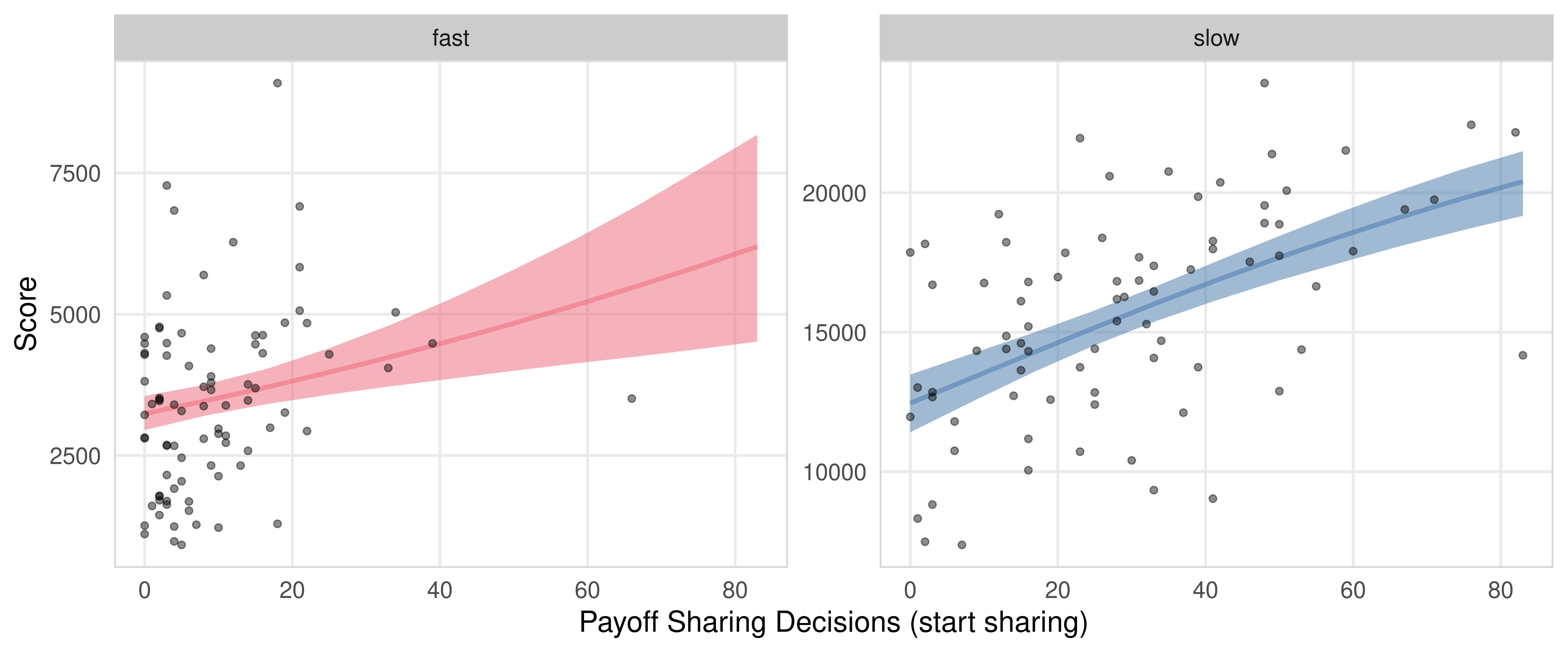
Model fitting (Group)
m.PayoffSharing.SwitchCounts.Group.data <- m.PayoffSharing.SwitchCounts.data %>%
  group_by(Group) %>%
  summarise(
    Score_0_1 = mean(Score_0_1),
    TrackingTime_0_1 = mean(TrackingTime_0_1),
    PCR_0_1 = mean(PCR_0_1),
    sum_n_switch_0_to_1 = sum(n_switch_0_to_1),
    ResourceSpeed = unique(ResourceSpeed)
  )  %>% mutate(c_sum_n_switch_0_to_1 = sum_n_switch_0_to_1 / max(sum_n_switch_0_to_1))

m.PayoffSharing.SwitchCounts.Score.Group.formula <- brmsformula(
  Score_0_1 ~ ResourceSpeed * c_sum_n_switch_0_to_1,
  phi ~ ResourceSpeed,
  family = Beta()
)

m.PayoffSharing.SwitchCounts.Score.Group.priors <-
    prior(normal(0, 0.5), class = b) +
    prior(normal(0, 1), class = Intercept) +
    prior(gamma(4, 0.1), class = Intercept, dpar = phi, lb = 0)
m.PayoffSharing.SwitchCounts.Score.Group.fit <- brm(
formula = m.PayoffSharing.SwitchCounts.Score.Group.formula,
data = m.PayoffSharing.SwitchCounts.Group.data,
prior = m.PayoffSharing.SwitchCounts.Score.Group.priors,
chains = 4,
cores = 4,
seed = 42,
iter = 2000,
file = paste0(fits_path, 'pyoff_sharing_count_score_group.rds'),
backend = "cmdstanr",
threads = threading(100),
save_pars = save_pars(all = TRUE)
)Model diagnostics
##  Family: beta
##   Links: mu = logit; phi = log
## Formula: Score_0_1 ~ ResourceSpeed * c_sum_n_switch_0_to_1
##          phi ~ ResourceSpeed
##    Data: m.PayoffSharing.SwitchCounts.Group.data (Number of observations: 36)
##   Draws: 4 chains, each with iter = 2000; warmup = 1000; thin = 1;
##          total post-warmup draws = 4000
##
## Regression Coefficients:
##                                         Estimate Est.Error l-95% CI u-95% CI Rhat Bulk_ESS Tail_ESS
## Intercept                                  -1.93      0.11    -2.14    -1.72 1.00     3284     2715
## phi_Intercept                               4.09      0.34     3.35     4.70 1.00     3156     2633
## ResourceSpeedslow                           1.47      0.19     1.10     1.86 1.00     2775     2713
## c_sum_n_switch_0_to_1                       0.81      0.35     0.13     1.48 1.00     3040     2798
## ResourceSpeedslow:c_sum_n_switch_0_to_1     1.00      0.37     0.26     1.71 1.00     2648     2741
## phi_ResourceSpeedslow                      -0.68      0.50    -1.66     0.32 1.00     2935     2746
##
## Draws were sampled using sample(hmc). For each parameter, Bulk_ESS
## and Tail_ESS are effective sample size measures, and Rhat is the potential
## scale reduction factor on split chains (at convergence, Rhat = 1).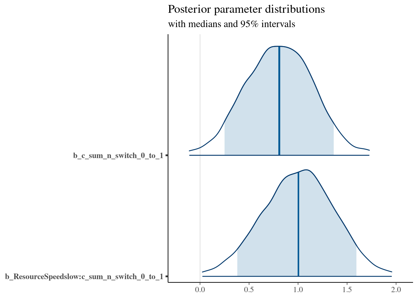
Figure
fig_payoff_sharing_switch_count_score_group <- m.PayoffSharing.SwitchCounts.Group.data %>%
  select(ResourceSpeed, c_sum_n_switch_0_to_1) %>%
  group_by() %>%
  data_grid(ResourceSpeed, c_sum_n_switch_0_to_1=seq(0, 1, 0.1)) %>%
  tidybayes::add_epred_draws(m.PayoffSharing.SwitchCounts.Score.Group.fit,
                             allow_new_levels = TRUE,
                             re_formula = NA) %>%
  ggplot(aes(x = c_sum_n_switch_0_to_1 * max(m.PayoffSharing.SwitchCounts.Group.data$sum_n_switch_0_to_1),
             y = .epred * empirical_max_score,
             color = ResourceSpeed,
             fill = ResourceSpeed)) +
  stat_lineribbon(aes(group = paste(group, ...width..)), .width = c(.9), alpha = 0.5) +
  scale_color_manual(breaks = c('fast', 'slow'),
                     aesthetics = c("colour", "fill"),
                    values = get_colors("Qual2", num.colors = 2, reverse = TRUE, gradient = FALSE),
                    guide = guide_legend(
                    title = "Resource",
                     )
                    ) +
  geom_point(
    data = m.PayoffSharing.SwitchCounts.Group.data,
    aes(x = sum_n_switch_0_to_1, y = Score_0_1 * empirical_max_score),  # , color = ResourceSpeed
    color = 'black',
    inherit.aes = FALSE,
    alpha = 0.45,
    size = 1.6
  ) +
  theme_clean() +
  panel_border() +
  facet_wrap(vars(ResourceSpeed), scales = "free") +
    theme(
    legend.position = "none", # "bottom",
  )  + labs(x = "Payoff Sharing Decisions (start sharing)", y = "Average Score (Group)", fill = "Resource", color = "Resource")

fig_payoff_sharing_switch_count_score_group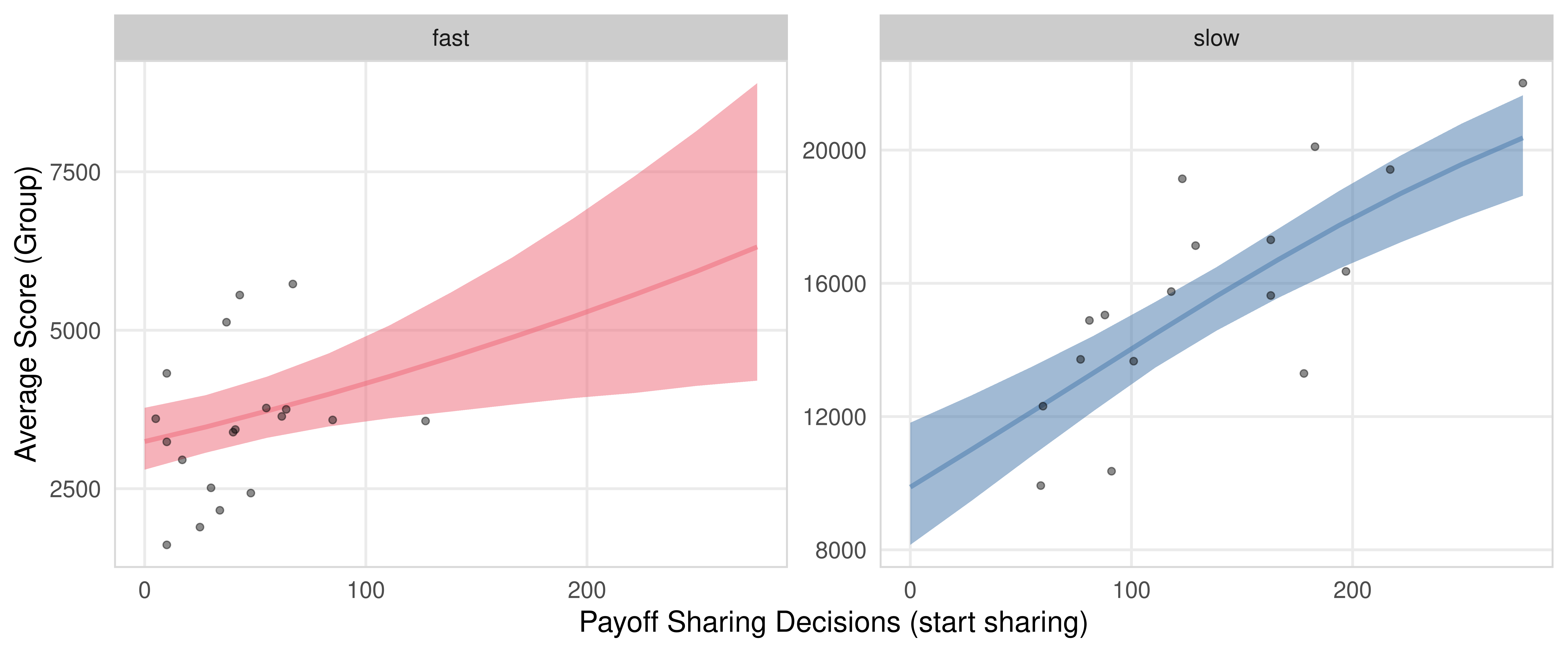
Total Sharing
total_sharing_time <- m.PayoffSharing.data %>%
  arrange(Participant, Time) %>%
  group_by(Participant) %>%
  summarise(
    total_sharing = sum(IsSignaling == 1, na.rm = TRUE),
    .groups = "drop"
  )

hist(total_sharing_time$total_sharing)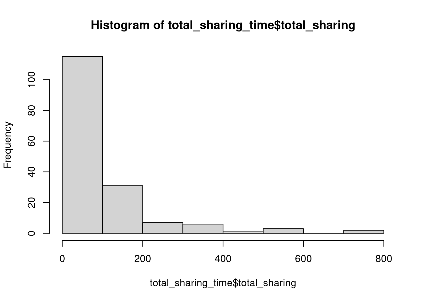
m.PayoffSharing.TotalSharing.data <- subj_data %>%
  filter(SignalingType == 'VP') %>%
  select(Participant, Group, ResourceSpeed, SignalingType, PCR, Score, TrackingTime) %>%
  left_join(total_sharing_time, by = "Participant") %>%
  mutate(PCR_0_1 = PCR / 40,
         Score_0_1 = Score / empirical_max_score,
         TrackingTime_0_1 = TrackingTime / 15.01,
         c_total_sharing = total_sharing / (15 * 60) + 0.01)
m.PayoffSharing.TotalSharing.data %>%
summarise(
n = n(),
max_time = max(total_sharing) / 60,
max_time = max(total_sharing) / (15 * 60)
)Total Sharing Model
m.PayoffSharing.TotalSharing.formula <- brmsformula(
  c_total_sharing ~ ResourceSpeed + (1 | Participant),
  family = Beta()
  )

m.PayoffSharing.TotalSharing.priors <-
    prior(normal(0, 0.5), class = b) +
    prior(normal(0, 1), class = Intercept)
Model fitting
m.PayoffSharing.TotalSharing.fit <- brm(
  formula = m.PayoffSharing.TotalSharing.formula,
  data    = m.PayoffSharing.TotalSharing.data,
  prior   = m.PayoffSharing.TotalSharing.priors,
  chains  = 4,
  cores   = 4,
  seed    = 42,
  iter    = 2000,
  file = paste0(fits_path, 'payoff_sharing_total_time_1.rds'),
  backend = "cmdstanr",
  threads = threading(100),
  control = list(adapt_delta = 0.95),
  save_pars = save_pars(all = TRUE)
  )
Model diagnostics
##  Family: beta
##   Links: mu = logit; phi = identity
## Formula: c_total_sharing ~ ResourceSpeed + (1 | Participant)
##    Data: m.PayoffSharing.TotalSharing.data (Number of observations: 165)
##   Draws: 4 chains, each with iter = 2000; warmup = 1000; thin = 1;
##          total post-warmup draws = 4000
##
## Multilevel Hyperparameters:
## ~Participant (Number of levels: 165)
##               Estimate Est.Error l-95% CI u-95% CI Rhat Bulk_ESS Tail_ESS
## sd(Intercept)     0.10      0.08     0.00     0.31 1.00     1473     1724
##
## Regression Coefficients:
##                   Estimate Est.Error l-95% CI u-95% CI Rhat Bulk_ESS Tail_ESS
## Intercept            -2.11      0.11    -2.34    -1.89 1.00     3921     2854
## ResourceSpeedslow     0.36      0.14     0.10     0.63 1.00     5701     3097
##
## Further Distributional Parameters:
##     Estimate Est.Error l-95% CI u-95% CI Rhat Bulk_ESS Tail_ESS
## phi     6.45      0.79     5.03     8.09 1.00     2985     1973
##
## Draws were sampled using sample(hmc). For each parameter, Bulk_ESS
## and Tail_ESS are effective sample size measures, and Rhat is the potential
## scale reduction factor on split chains (at convergence, Rhat = 1).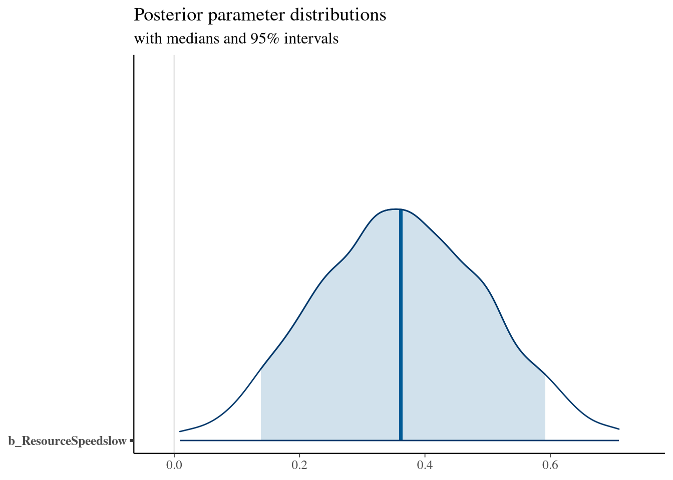
Condition draws
m.PayoffSharing.TotalSharing.fit %>%
  emmeans(~ ResourceSpeed, epred = TRUE, type = "response", re_formula = NA) %>%
  gather_emmeans_draws() %>%
  mutate(.value = .value * 15) %>%  # convert to minutes
  ggdist::mean_hdci(.width = 0.9) %>%
knitr::kable("html", digits = 2) %>% kable_classic(full_width = T, position = "center", )| ResourceSpeed | .value | .lower | .upper | .width | .point | .interval |
|---|---|---|---|---|---|---|
| fast | 1.63 | 1.35 | 1.89 | 0.9 | mean | hdci |
| slow | 2.23 | 1.91 | 2.58 | 0.9 | mean | hdci |
Total Sharing vs Score Model
m.PayoffSharing.TotalSharing.data %>%
  ggplot(aes(x=c_total_sharing, y=Score, color=ResourceSpeed)) +
  facet_wrap(vars(ResourceSpeed), scales="free") +
  geom_point() +
  geom_smooth(method="lm")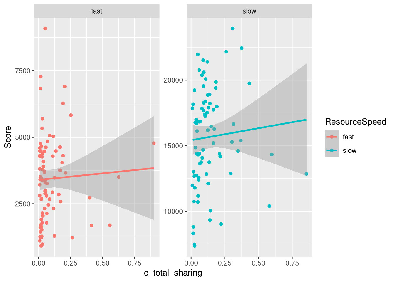
m.PayoffSharing.TotalSharing.data %>%
  group_by(Group) %>%
  summarise(
    Score_0_1 = mean(Score),
    TrackingTime_0_1 = mean(TrackingTime_0_1),
    PCR_0_1 = mean(PCR_0_1),
    sum_total_sharing = sum(total_sharing),
    ResourceSpeed = unique(ResourceSpeed)
  ) %>%
  mutate(sum_total_sharing = sum_total_sharing / max(sum_total_sharing)) %>%
  ggplot(aes(x=sum_total_sharing, y=Score_0_1, color=ResourceSpeed)) +
  facet_wrap(vars(ResourceSpeed), scales="free") +
  geom_point() +
  geom_smooth(method="lm")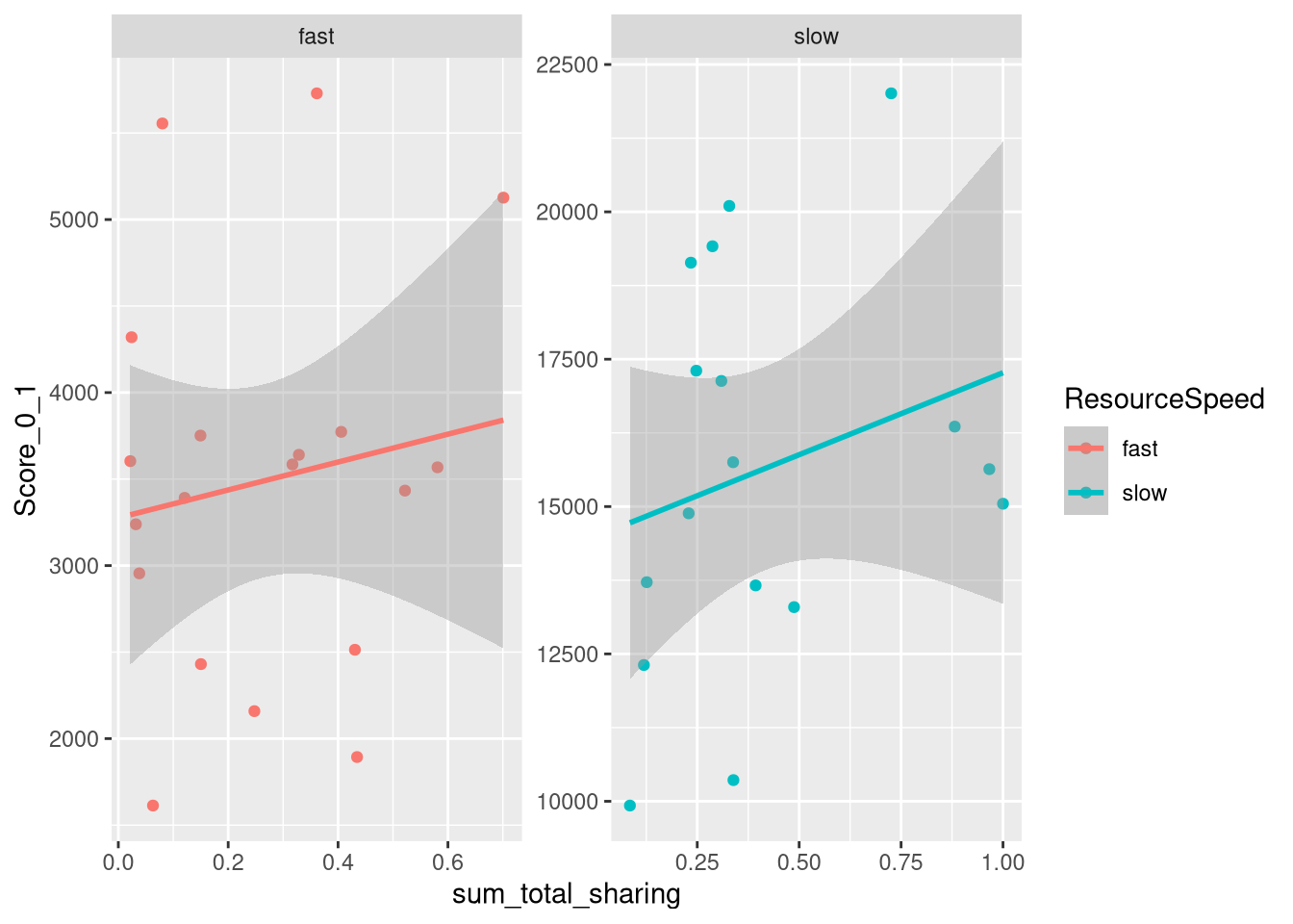
Model fitting (Participant)
m.PayoffSharing.TotalSharing.Score.formula <- brmsformula(
  Score_0_1 ~ ResourceSpeed * c_total_sharing,
  phi ~ ResourceSpeed,
  family = Beta()
)

m.PayoffSharing.TotalSharing.Score.priors <-
    prior(normal(0, 0.5), class = b) +
    prior(normal(0, 1), class = Intercept) +
    prior(gamma(4, 0.1), class = Intercept, dpar = phi, lb = 0)
m.PayoffSharing.TotalSharing.Score.fit <- brm(
formula = m.PayoffSharing.TotalSharing.Score.formula,
data = m.PayoffSharing.TotalSharing.data,
prior = m.PayoffSharing.TotalSharing.Score.priors,
chains = 4,
cores = 4,
seed = 42,
iter = 2000,
file = paste0(fits_path, 'payoff_sharing_total_time_score.rds'),
backend = "cmdstanr",
threads = threading(100),
save_pars = save_pars(all = TRUE)
)Model diagnostics
##  Family: beta
##   Links: mu = logit; phi = log
## Formula: Score_0_1 ~ ResourceSpeed * c_total_sharing
##          phi ~ ResourceSpeed
##    Data: m.PayoffSharing.TotalSharing.data (Number of observations: 165)
##   Draws: 4 chains, each with iter = 2000; warmup = 1000; thin = 1;
##          total post-warmup draws = 4000
##
## Regression Coefficients:
##                                   Estimate Est.Error l-95% CI u-95% CI Rhat Bulk_ESS Tail_ESS
## Intercept                            -1.85      0.06    -1.97    -1.71 1.00     4934     2748
## phi_Intercept                         3.38      0.16     3.04     3.68 1.00     5764     3068
## ResourceSpeedslow                     2.20      0.10     2.00     2.40 1.00     4509     3139
## c_total_sharing                       0.14      0.27    -0.42     0.69 1.00     5446     3019
## ResourceSpeedslow:c_total_sharing     0.30      0.38    -0.44     1.06 1.00     4275     3171
## phi_ResourceSpeedslow                -1.09      0.22    -1.51    -0.66 1.00     5572     3031
##
## Draws were sampled using sample(hmc). For each parameter, Bulk_ESS
## and Tail_ESS are effective sample size measures, and Rhat is the potential
## scale reduction factor on split chains (at convergence, Rhat = 1).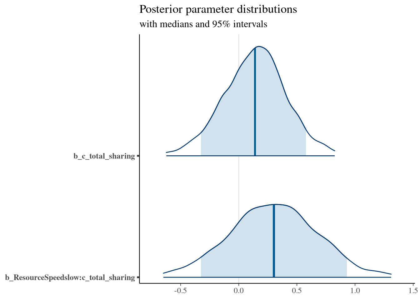
Model fitting (Group)
m.PayoffSharing.TotalSharing.Group.data <- m.PayoffSharing.TotalSharing.data %>%
  group_by(Group) %>%
  summarise(
    Score_0_1 = mean(Score_0_1),
    TrackingTime_0_1 = mean(TrackingTime_0_1),
    PCR_0_1 = mean(PCR_0_1),
    sum_total_sharing = sum(total_sharing),
    ResourceSpeed = unique(ResourceSpeed)
  )  %>% mutate(c_sum_total_sharing = sum_total_sharing / max(sum_total_sharing))

m.PayoffSharing.TotalSharing.Score.Group.formula <- brmsformula(
  Score_0_1 ~ ResourceSpeed * c_sum_total_sharing,
  phi ~ ResourceSpeed,
  family = Beta()
)

m.PayoffSharing.TotalSharing.Score.Group.priors <-
    prior(normal(0, 0.5), class = b) +
    prior(normal(0, 1), class = Intercept) +
    prior(gamma(4, 0.1), class = Intercept, dpar = phi, lb = 0)
m.PayoffSharing.TotalSharing.Score.Group.fit <- brm(
formula = m.PayoffSharing.TotalSharing.Score.Group.formula,
data = m.PayoffSharing.TotalSharing.Group.data,
prior = m.PayoffSharing.TotalSharing.Score.Group.priors,
chains = 4,
cores = 4,
seed = 42,
iter = 2000,
file = paste0(fits_path, 'payoff_sharing_total_time_score_group.rds'),
backend = "cmdstanr",
threads = threading(100),
save_pars = save_pars(all = TRUE)
)Model diagnostics
##  Family: beta
##   Links: mu = logit; phi = log
## Formula: Score_0_1 ~ ResourceSpeed * c_sum_total_sharing
##          phi ~ ResourceSpeed
##    Data: m.PayoffSharing.TotalSharing.Group.data (Number of observations: 36)
##   Draws: 4 chains, each with iter = 2000; warmup = 1000; thin = 1;
##          total post-warmup draws = 4000
##
## Regression Coefficients:
##                                       Estimate Est.Error l-95% CI u-95% CI Rhat Bulk_ESS Tail_ESS
## Intercept                                -1.83      0.12    -2.06    -1.58 1.00     3636     3390
## phi_Intercept                             3.98      0.36     3.19     4.61 1.00     3828     2614
## ResourceSpeedslow                         1.86      0.21     1.42     2.27 1.00     2791     2589
## c_sum_total_sharing                       0.17      0.30    -0.41     0.76 1.00     3666     2802
## ResourceSpeedslow:c_sum_total_sharing     0.53      0.36    -0.19     1.23 1.00     2850     2566
## phi_ResourceSpeedslow                    -1.47      0.51    -2.47    -0.45 1.00     3148     2794
##
## Draws were sampled using sample(hmc). For each parameter, Bulk_ESS
## and Tail_ESS are effective sample size measures, and Rhat is the potential
## scale reduction factor on split chains (at convergence, Rhat = 1).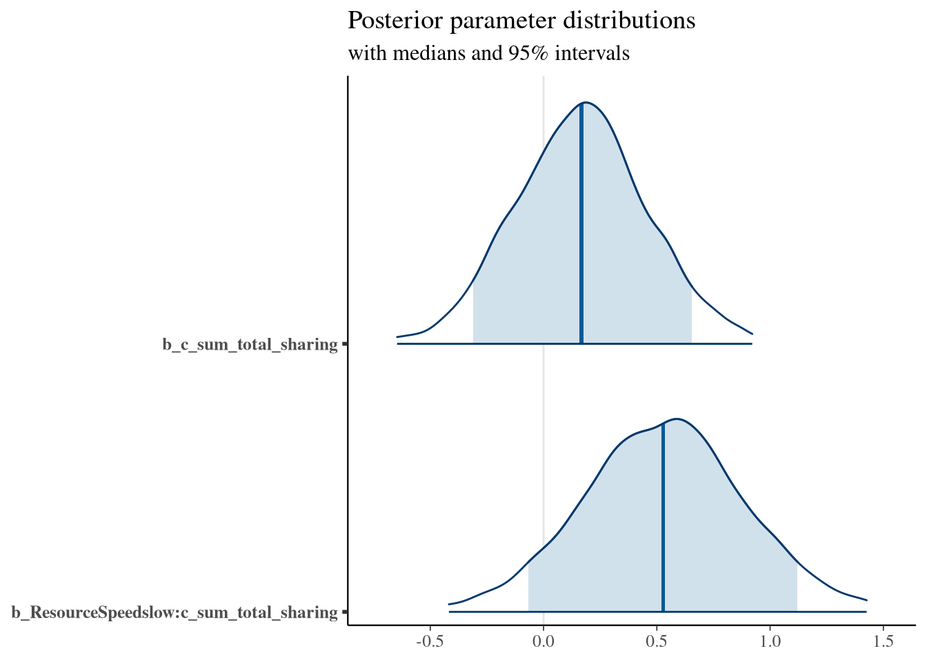
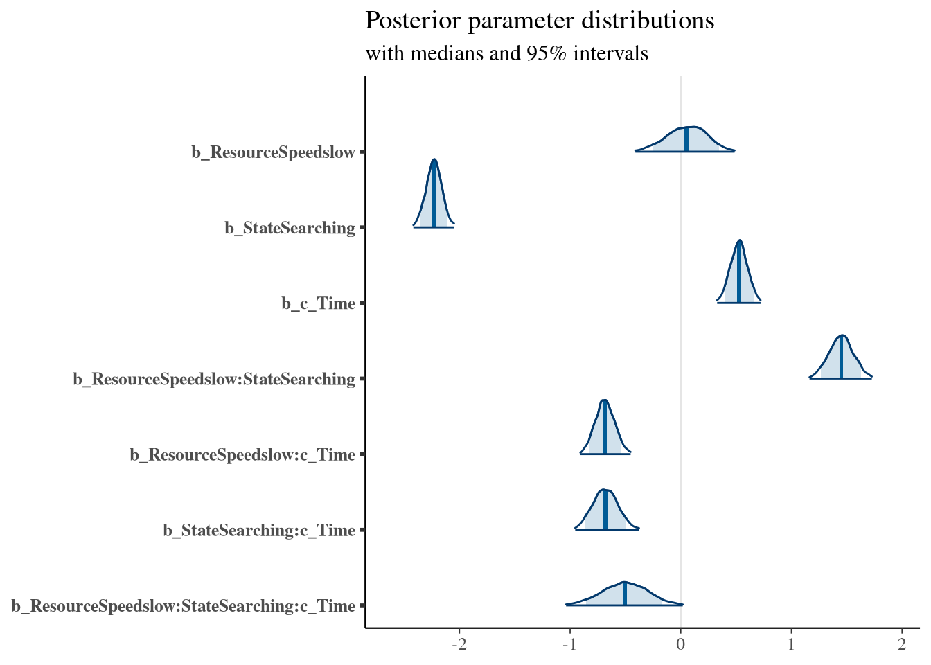
Sharing Probability: Resource, State, Time, Distance
m.PayoffSharing.1.formula <- brmsformula(
  IsSignaling ~ ResourceSpeed * State * c_Time + (1 | Participant),
  family = bernoulli(link = "logit")
)m.PayoffSharing.1.priors <-
prior(normal(0, 0.5), class = b) +
prior(normal(0, 0.1), class = 'sd') +
prior(normal(0, 1), class = Intercept)Model fitting
m.PayoffSharing.1.fit <- brm(
formula = m.PayoffSharing.1.formula,
data = m.PayoffSharing.data,
prior = m.PayoffSharing.1.priors,
chains = 4,
cores = 4,
seed = 42,
iter = 2000,
file = paste0(fits_path, 'payoff_sharing_probability_1.rds'),
backend = "cmdstanr",
threads = threading(100),
control = list(adapt_delta = 0.95),
save_pars = save_pars(all = TRUE)
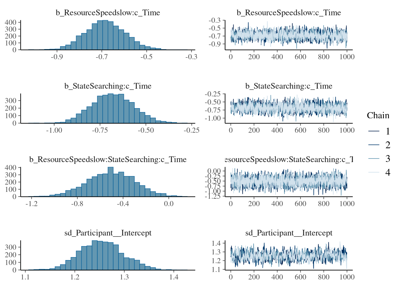
)Model diagnostics
##  Family: bernoulli
##   Links: mu = logit
## Formula: IsSignaling ~ ResourceSpeed * State * c_Time + (1 | Participant)
##    Data: m.PayoffSharing.data (Number of observations: 138025)
##   Draws: 4 chains, each with iter = 2000; warmup = 1000; thin = 1;
##          total post-warmup draws = 4000
##
## Multilevel Hyperparameters:
## ~Participant (Number of levels: 165)
##               Estimate Est.Error l-95% CI u-95% CI Rhat Bulk_ESS Tail_ESS
## sd(Intercept)     1.25      0.04     1.17     1.34 1.00      562     1139
##
## Regression Coefficients:
##                                         Estimate Est.Error l-95% CI u-95% CI Rhat Bulk_ESS Tail_ESS
## Intercept                                  -2.19      0.14    -2.47    -1.92 1.02      255      590
## ResourceSpeedslow                           0.05      0.18    -0.31     0.39 1.01      218      498
## StateSearching                             -2.23      0.07    -2.37    -2.09 1.00     2203     2780
## c_Time                                      0.53      0.08     0.38     0.68 1.00     1949     2896
## ResourceSpeedslow:StateSearching            1.45      0.11     1.23     1.67 1.00     2450     2987
## ResourceSpeedslow:c_Time                   -0.68      0.09    -0.86    -0.51 1.00     1930     2887
## StateSearching:c_Time                      -0.68      0.11    -0.90    -0.45 1.00     2004     2896
## ResourceSpeedslow:StateSearching:c_Time    -0.51      0.21    -0.91    -0.10 1.00     2747     3326
##
## Draws were sampled using sample(hmc). For each parameter, Bulk_ESS
## and Tail_ESS are effective sample size measures, and Rhat is the potential
## scale reduction factor on split chains (at convergence, Rhat = 1).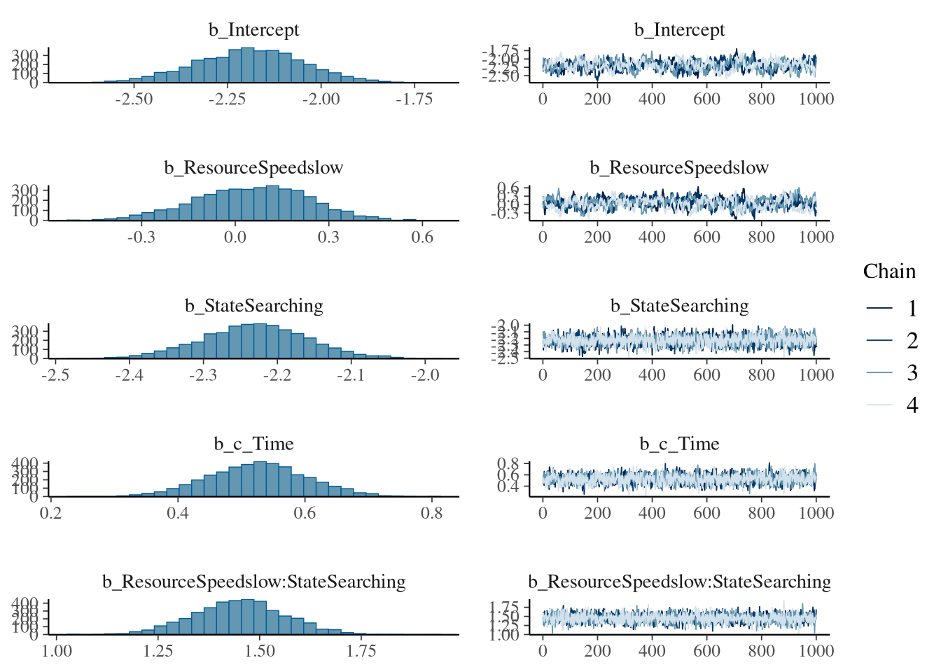

Figure
fig_payoff_sharing_resource_time_state <- m.PayoffSharing.data %>%
  select(Participant, State, ResourceSpeed, IsSignaling) %>%
  group_by() %>%
  data_grid(ResourceSpeed, State, c_Time=seq(0, 1, 0.1)) %>%
  tidybayes::add_epred_draws(m.PayoffSharing.1.fit,
                             allow_new_levels = TRUE,
                             re_formula = NA) %>%
  ggplot(aes(x = c_Time * 15,
             y = .epred,
             color = ResourceSpeed,
             fill = ResourceSpeed)) +
  stat_lineribbon(aes(group = paste(group, ...width..)), .width = c(.9), alpha = 0.5) +
  scale_color_manual(breaks = c('fast', 'slow'),
                     aesthetics = c("colour", "fill"),
                    values = get_colors("Qual2", num.colors = 2, reverse = TRUE, gradient = FALSE),
                    guide = guide_legend(
                    title = "Resource",
                     )
                    ) +
  theme_clean() +
  panel_border() +
  facet_wrap(vars(State)) +
    theme(
    legend.position = "none", # "bottom",
  ) +
  labs(x = "Time [m]", y = "Payoff Sharing Probability", fill = "Resource", color = "Resource")

fig_payoff_sharing_resource_time_state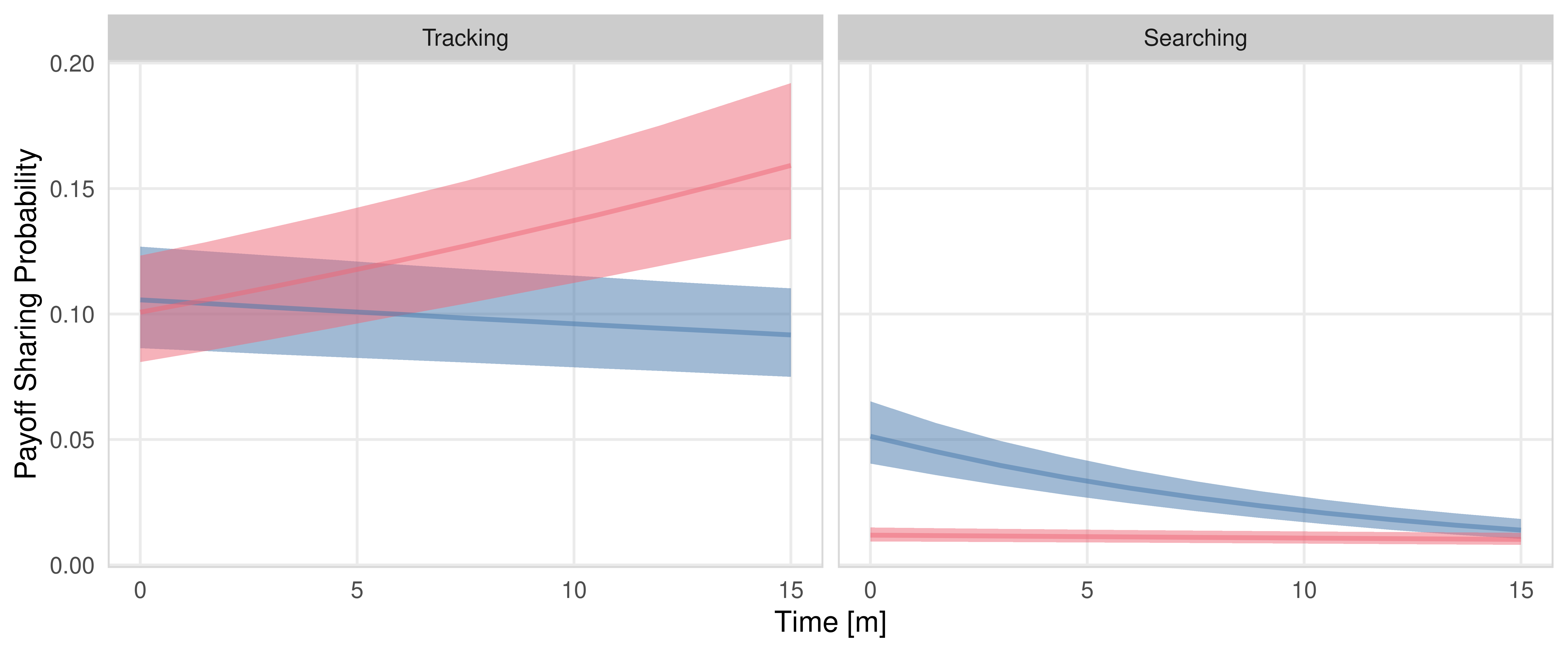
Statistical Comparisons
m.PayoffSharing.1.fit %>%
  emmeans(~ ResourceSpeed * State,
          epred = TRUE,
          type = "response") %>%
  contrast(method = "pairwise", simple = "each", combine = TRUE) %>%
  gather_emmeans_draws() %>%
  mean_hdci(.width = 0.9) %>%
  mutate(.value = round(.value, 2), .lower = round(.lower, 2), .upper = round(.upper, 2)) %>%
  kable("html", digits = 2) %>%
kable_classic(full_width = T, position = "center")| State | ResourceSpeed | contrast | .value | .lower | .upper | .width | .point | .interval |
|---|---|---|---|---|---|---|---|---|
| . | fast | Tracking - Searching | 0.12 | 0.10 | 0.14 | 0.9 | mean | hdci |
| . | slow | Tracking - Searching | 0.07 | 0.06 | 0.09 | 0.9 | mean | hdci |
| Searching | . | fast - slow | -0.02 | -0.02 | -0.01 | 0.9 | mean | hdci |
| Tracking | . | fast - slow | 0.03 | 0.00 | 0.06 | 0.9 | mean | hdci |
m.PayoffSharing.1.fit %>%
  emmeans(~ ResourceSpeed * State * c_Time,
          at = list(c_Time = c(0, 1)),
          epred = TRUE,
          type = "response") %>%
  contrast(method = "revpairwise", simple = "each", combine = TRUE) %>%
  gather_emmeans_draws() %>%
  mean_hdci(.width = 0.9) %>%
  mutate(.value = round(.value, 2), .lower = round(.lower, 2), .upper = round(.upper, 2)) %>%
  kable("html", digits = 2) %>%
kable_classic(full_width = T, position = "center")| State | c_Time | ResourceSpeed | contrast | .value | .lower | .upper | .width | .point | .interval |
|---|---|---|---|---|---|---|---|---|---|
| . | 0 | fast | Searching - Tracking | -0.09 | -0.11 | -0.07 | 0.9 | mean | hdci |
| . | 0 | slow | Searching - Tracking | -0.05 | -0.07 | -0.04 | 0.9 | mean | hdci |
| . | 1 | fast | Searching - Tracking | -0.15 | -0.18 | -0.12 | 0.9 | mean | hdci |
| . | 1 | slow | Searching - Tracking | -0.08 | -0.09 | -0.06 | 0.9 | mean | hdci |
| Searching | . | fast | c_Time1 - c_Time0 | 0.00 | 0.00 | 0.00 | 0.9 | mean | hdci |
| Searching | . | slow | c_Time1 - c_Time0 | -0.04 | -0.05 | -0.03 | 0.9 | mean | hdci |
| Searching | 0 | . | slow - fast | 0.04 | 0.03 | 0.05 | 0.9 | mean | hdci |
| Searching | 1 | . | slow - fast | 0.00 | 0.00 | 0.01 | 0.9 | mean | hdci |
| Tracking | . | fast | c_Time1 - c_Time0 | 0.06 | 0.04 | 0.08 | 0.9 | mean | hdci |
| Tracking | . | slow | c_Time1 - c_Time0 | -0.01 | -0.02 | -0.01 | 0.9 | mean | hdci |
| Tracking | 0 | . | slow - fast | 0.00 | -0.02 | 0.03 | 0.9 | mean | hdci |
| Tracking | 1 | . | slow - fast | -0.07 | -0.10 | -0.03 | 0.9 | mean | hdci |
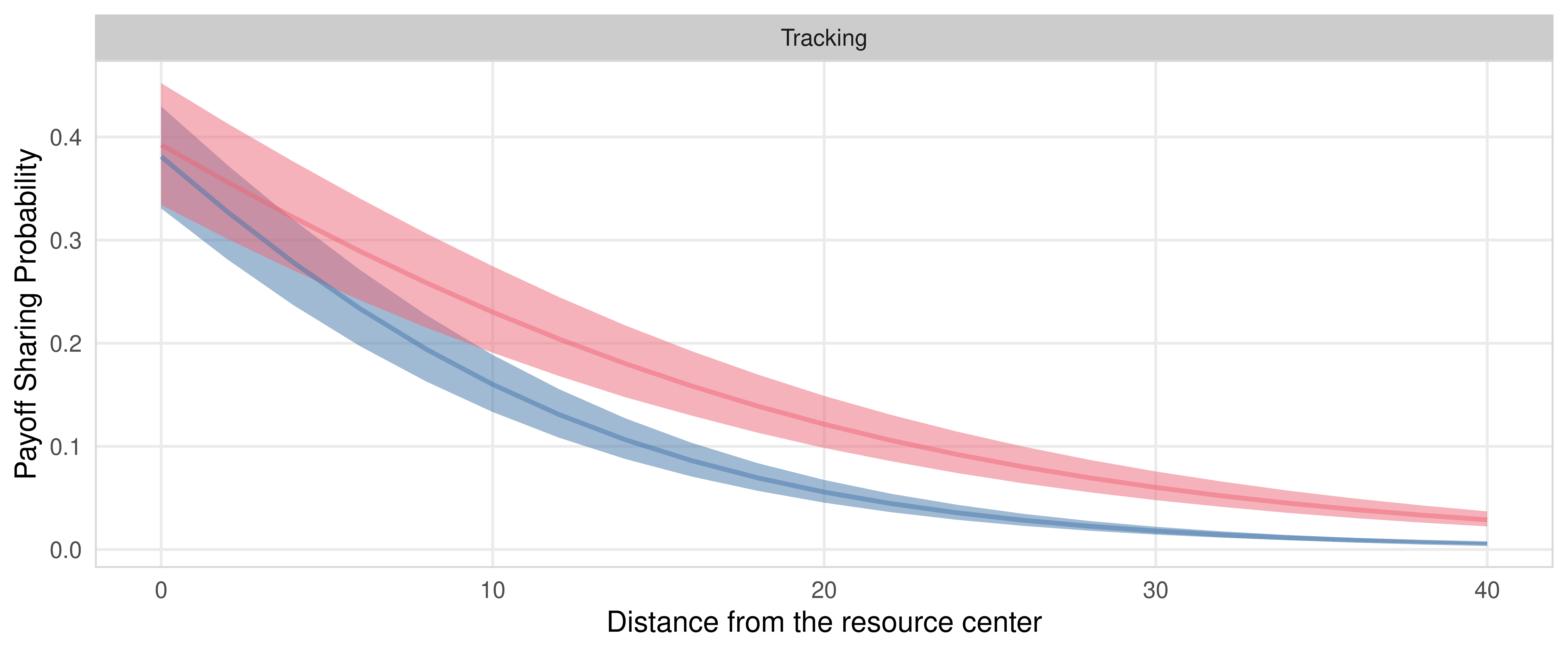
Sharing Probability: Resource, Distance
m.PayoffSharing.2.data <- m.PayoffSharing.data %>%
  filter(State == 'Tracking', c_OwnDistFromResource <= 1) %>%
  mutate(OwnDistFromResourceInt = round(OwnDistFromResource))


m.PayoffSharing.2.formula <- brmsformula(
  IsSignaling ~ ResourceSpeed * c_OwnDistFromResource + (1 | Participant),
  family = bernoulli(link = "logit")
)m.PayoffSharing.2.priors <-
prior(normal(0, 0.5), class = b) +
prior(normal(0, 0.1), class = 'sd') +
prior(normal(0, 1), class = Intercept)m.PayoffSharing.2.data %>%
ggplot(aes(x = c_OwnDistFromResource, y=IsSignaling, color=ResourceSpeed)) +
geom_smooth()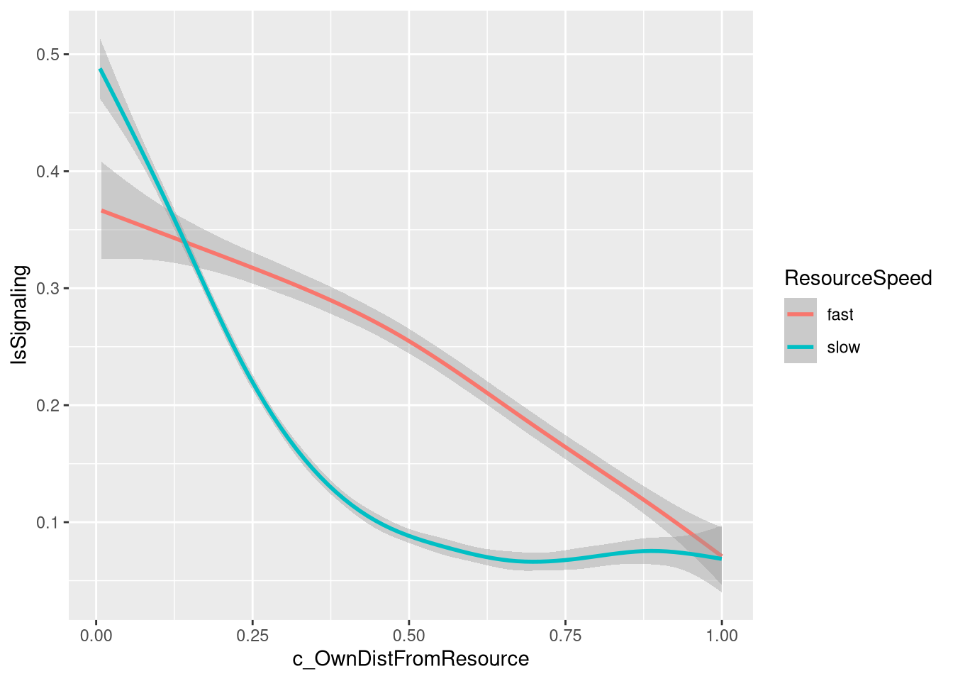
Model fitting
m.PayoffSharing.2.fit <- brm(
  formula = m.PayoffSharing.2.formula,
  data    = m.PayoffSharing.2.data,
  prior   = m.PayoffSharing.2.priors,
  chains  = 4,
  cores   = 4,
  seed    = 42,
  iter    = 2000,
  file = paste0(fits_path, 'payoff_sharing_probability_distance_1.rds'),
  backend = "cmdstanr",
  threads = threading(100),
  control = list(adapt_delta = 0.95),
  save_pars = save_pars(all = TRUE)
  )
Model diagnostics
##  Family: bernoulli
##   Links: mu = logit
## Formula: IsSignaling ~ ResourceSpeed * c_OwnDistFromResource + (1 | Participant)
##    Data: m.PayoffSharing.2.data (Number of observations: 73938)
##   Draws: 4 chains, each with iter = 2000; warmup = 1000; thin = 1;
##          total post-warmup draws = 4000
##
## Multilevel Hyperparameters:
## ~Participant (Number of levels: 165)
##               Estimate Est.Error l-95% CI u-95% CI Rhat Bulk_ESS Tail_ESS
## sd(Intercept)     1.33      0.04     1.24     1.41 1.00      523     1266
##
## Regression Coefficients:
##                                         Estimate Est.Error l-95% CI u-95% CI Rhat Bulk_ESS Tail_ESS
## Intercept                                  -0.44      0.15    -0.74    -0.15 1.01      247      556
## ResourceSpeedslow                          -0.05      0.19    -0.44     0.31 1.02      146      377
## c_OwnDistFromResource                      -3.08      0.11    -3.29    -2.88 1.00     2142     3021
## ResourceSpeedslow:c_OwnDistFromResource    -1.60      0.13    -1.86    -1.34 1.00     2233     2763
##
## Draws were sampled using sample(hmc). For each parameter, Bulk_ESS
## and Tail_ESS are effective sample size measures, and Rhat is the potential
## scale reduction factor on split chains (at convergence, Rhat = 1).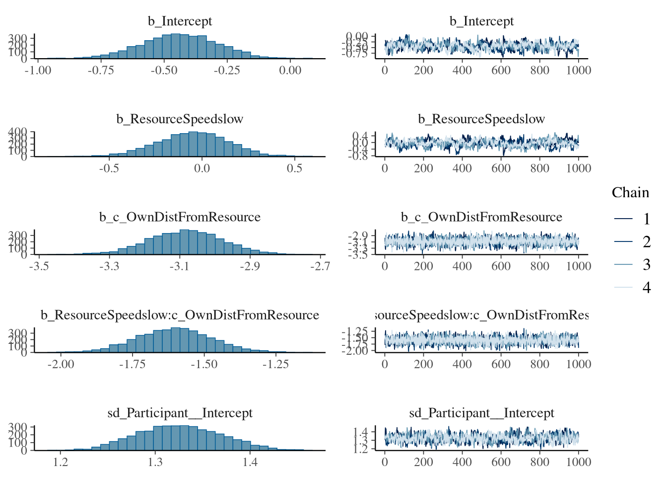
Figure
fig_payoff_sharing_resource_distance <- m.PayoffSharing.2.data %>%
  select(Participant, State, ResourceSpeed, c_OwnDistFromResource, IsSignaling) %>%
  group_by() %>%
  data_grid(ResourceSpeed, State="Tracking", c_OwnDistFromResource=seq(0, 1, 0.05)) %>%
  tidybayes::add_epred_draws(m.PayoffSharing.2.fit,
                             allow_new_levels = TRUE,
                             re_formula = NA) %>%
  ggplot(aes(x = c_OwnDistFromResource * 40,
             y = .epred,
             color = ResourceSpeed,
             fill = ResourceSpeed)) +
  stat_lineribbon(aes(group = paste(group, ...width..)), .width = c(.9), alpha = 0.5) +
  scale_color_manual(breaks = c('fast', 'slow'),
                     aesthetics = c("colour", "fill"),
                    values = get_colors("Qual2", num.colors = 2, reverse = TRUE, gradient = FALSE),
                    guide = guide_legend(
                    title = "Resource",
                     )
                    ) +
  theme_clean() +
  panel_border() +
  facet_wrap(vars(State)) +
    theme(
    legend.position = "none", # "bottom",
  ) +
  labs(x = "Distance from the resource center", y = "Payoff Sharing Probability", fill = "Resource", color = "Resource")

fig_payoff_sharing_resource_distance